2.c Eratosthenes and the Flat Earth model

A reader has pointed out that we can also use the data collected in our Eratosthenes experiment to test the hypothesis that the Earth is flat and that the difference in shadows is caused by the sun being a relatively small distance from the flat Earth. And we can compare this test to a test of our round Earth hypothesis.

If the Earth is flat, and we make an observation like Eratosthenes, that a vertical stick in one location casts no shadow, while a vertical stick some distance north (or south) does cast a shadow, then we can use geometry to figure out how far away the sun must be.

Distance to the sun in a flat Earth model

Using similar triangles to determine the distance from a flat Earth to the sun, given an observation of the shadow of a vertical stick, and knowing the distance from a point where the sun is overhead.

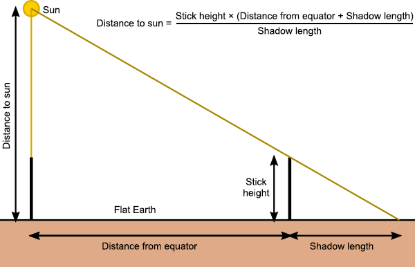
If the Earth is indeed flat then when we do this calculation for each of our 19 observations we should get the same answer, to within any experimental error. In particular, there should be no systematic difference in our answers that depends on the distance from the equator. Analogously, in our round Earth model, the circumference we have calculated for the Earth from each of our observations should also be the same to within experimental errors, and show no systematic difference depending on distance from the equator.

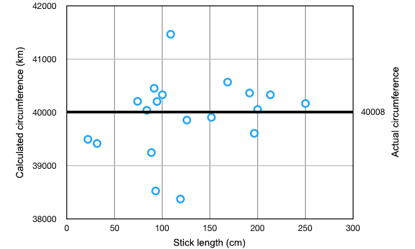
So let’s test those things! Here are graphs of the results, on which I’ve included a linear least squares best fit line, showing the line’s equation and statistical R2 score. The R2 value, or coefficient of determination, is a measure of how likely the data values (the circumference of the Earth in the round Earth hypothesis, or the distance to the sun in the flat Earth hypothesis) are to be correlated with the fixed values (the distance from the equator in both cases). We’ll discuss that after we see the data.

Earth's circumference versus distance from equator

Plot of 19 measurements of the Earth’s circumference, assuming the round Earth model, versus distance from the equator.

Distance to sun versus distance from equator

Plot of 19 measurements of the distance of the sun from Earth, assuming the flat Earth model, versus distance from the equator.

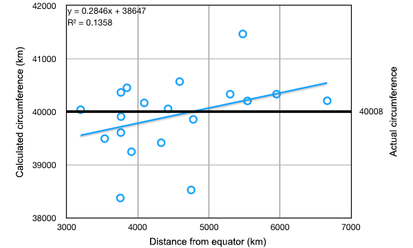
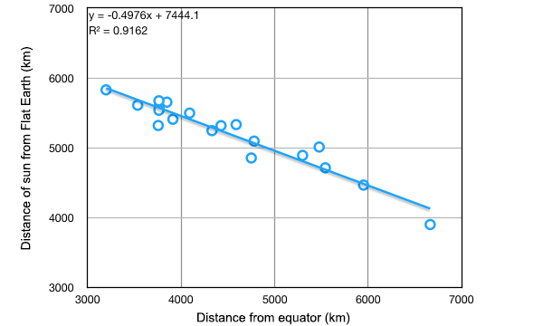
The first thing to notice is that in the top plot, the circumference of the Earth values look fairly evenly scattered around the true value. In the bottom plot, the calculated values for the distance of the sun from Earth are not evenly scattered; they show a pretty clear trend of giving larger distances for the data points closer to the equator and smaller distances for data points further from the equator. We can quantify this by looking at the straight line fits to the data and in particular the R2 value.

To do a rigorous statistical test, we need to set up our two possible null hypotheses. These are statements that for the purpose of our statistical test we assume are true, and then we calculate the probability that what we observe could happen by random chance. Our two null hypotheses are:

1. For the spherical Earth model, the calculated circumference of Earth is independent of the distance from the equator of our data points.

2. For the flat Earth model, the calculated distance of the sun from Earth is independent of the distance from the equator of our data points.

To test these, we use a probability distribution that tells us how likely our observed R2 scores are. An appropriate one to use is Student’s t-distribution. We calculate Student’s t-distribution function for 19 data points and 2 degrees of freedom (the y-intercept and the slope of our fitted line), determine a value for the function below which 95% of the probability distribution lies, and convert this to an R2 value using the known transformation. In simpler terms (TL;DR), we’re working out a number R2(P<0.05) which, if our calculated values are independent of distance from the equator, then we would expect 95% of experiments to give an R2 value less than the number R2(P<0.05).

Doing the maths, our value for R2(P<0.05) is 0.334. What this means is that if our R2 value is greater than 0.334, then we should reject our null hypothesis – the data are statistically inconsistent with the hypothesis (at the 95% confidence level, for those who like statistical rigour*). On the other hand, if our R2 value is less than 0.334, we cannot reject our null hypothesis – we haven’t proven it to be true, we have just shown that our data are consistent with it.

Now let’s look at our calculated R2 values. For the spherical Earth hypothesis, R2 = 0.1358. This is less than the critical value, so our data are consistent with our hypothesis. In contrast, for the flat Earth model, R2 = 0.9162. This is greater than the critical value, so we can confidently reject the flat Earth hypothesis as inconsistent with our experiment!

So there you have it. Not only did we successfully measure the circumference of the Earth to within our experimental errors, we have now also shown that our experimental results are consistent with a spherical Earth model, and inconsistent with a flat Earth model.

* Note: Choosing the 95% confidence level is typical for statistical hypothesis testing. You should always choose your confidence level before performing the calculations, to avoid any bias in your reporting. You can choose other levels, such as 99%. If I’d done that, we would have found that our data are also inconsistent with the flat Earth model at the more stringent 99% confidence level. In fact, calculating backwards, the confidence level of our rejection is a bit above 99.7%.

8. Earth’s magnetic field

Magnetic fields have both a strength and a direction at each point in space. The strength is a measure of how strong a force a magnet feels when in the field, and the direction is the direction of the force on a magnetic north pole. North poles of magnets on Earth tend to be pulled towards the Earth’s North Magnetic Pole (which is in fact a magnetic south pole, but called “the North Magnetic Pole” because it is in the northern hemisphere), while south poles are pulled towards the South Magnetic Pole (similarly, actually a magnetic north pole, called “the South Magnetic Pole” because it’s in the south). Humans have used this property of magnets for thousands of years to navigate, with magnetic compasses.

The simplest magnetic field is what’s known as a dipole, because it has two poles: a north pole and a south pole. You can think of this as the magnetic field of a simple bar magnet. The magnetic field lines are loops, with the field direction pointing out of the north pole and into the south pole, and the loops closing inside of the magnet.

A magnetic dipole

Illustration of magnetic field lines around a magnetic dipole. The north and south poles of the magnet are marked.

It’s straightforward to measure both the strength and the direction of the Earth’s magnetic field at any point on the surface, using a device known as a magnetometer. So what does it look like? Here are some contour maps showing the Earth’s magnetic field strength and the inclination – the angle the field lines make to the ground.

Earth's magnetic field intensity

Earth’s magnetic field strength. The minimum field strength occurs over South America; the maximum field strengths occur just off Antarctica, south of Australia, and in the broad patch covering both central Russia and northern Canada. (Public domain image by the US National Ocean and Atmospheric Administration.)

Earth's magnetic field inclination

Earth’s magnetic field inclination. The field direction is parallel to the ground at points along the green line, points into the ground in the red region, and points out of the ground in the blue region. The field emerges vertically at the white mark off the coast of Antarctica, south of Australia – this is the Earth’s South Magnetic Pole. The field points straight down at the North Magnetic Pole, north of Canada – not shown in this Mercator projection map, which omits areas with latitude greater than 70° north or south. (Public domain image by the US National Ocean and Atmospheric Administration.)

Now, how can we explain these observations with either a spherical Earth or flat Earth model? Let’s start with the spherical model.

You may notice a few things about the maps above. The Earth’s magnetic field is not symmetrical at the surface. The lowest intensity point over South America is not mirrored anywhere in the northern hemisphere. And the South Magnetic Pole is at a latitude about 64°S, while the North Magnetic Pole is at latitude 82°N. As it happens, this observed magnetic field is to a first approximation the field of a magnetic dipole – just not a dipole that is centred at the centre of the Earth. The dipole is tilted with respect to Earth’s rotation, and is offset a bit to one side – towards south-east Asia and away from South America. This explains the minimum intensity in South America, and the asymmetry of the magnetic poles.

A magnetic dipole

The Earth’s magnetic field is approximated by a dipole, offset from the centre of the Earth. The rotational axis is the light blue line, with geographic north and south poles marked. The red dots are the equivalent magnetic poles. The North Magnetic Pole is much closer to the geographic north pole than the South Magnetic Pole is to the geographic south pole. (As stated in the text, the “North Magnetic Pole” of the Earth is actually a magnetic south pole, and vice versa.)

Models of the interior of the Earth suggest that there are circulating electrical currents in the molten core, which is composed mostly of iron. These currents are caused by thermal convection, and twisted into helices by the Coriolis force produced by the Earth’s rotation, both well understood physical processes. Circulating electrical currents are exactly what causes magnetic fields. The simplest version of this so-called dynamo theory model is one in which there is a single giant loop of current, generating a simple magnetic dipole. And in fact this dipole fits the Earth’s magnetic field to an average deviation of 16% [1].

This is not a perfect fit, but it’s not too bad. The adjustments needed to better fit Earth’s measured field are relatively small, and can also be understood as the effects of circulating currents in the Earth’s core, causing additional components of the field with smaller magnitudes. (The Earth’s magnetic field also changes over time, but we’ll discuss that another day: Now available in Proof 44. Magnetic striping.)

If the Earth is flat, however, there is no such relatively simple way to understand the strength and direction of Earth’s magnetic field using standard electromagnetic theory. Even the gross overall structure—which is readily explained by a magnetic dipole for the spherical Earth—has no such simple explanation. The shape of the field on a flat Earth would require either multiple electrical dynamos or large deposits of magnetic materials under the Earth’s crust, and they would have to be fortuitously arranged in such a way that they closely mimic a dipole if we assumed the Earth to be a sphere. For any random arrangement of magnetic field-inducing structures on a flat Earth to happen to mimic the field of a spherical planet so closely is highly unlikely. Potentially it could happen, but the Earth actually being a sphere is a much more likely explanation.

That the simpler model is more likely to be true than the one requiring many ad-hoc assumptions is a case of Occam’s razor. In science, particularly, a simpler theory is more easily testable than one with a large number of ad-hoc assumptions. Occam’s razor will come up a lot, and I should probably write a sidebar article about it.

References:

[1] Nevalainen, J.; Usoskin, I.G.; Mishev, A. “Eccentric dipole approximation of the geomagnetic field: Application to cosmic ray computations”. Advances in Space Research, 52, p. 22-29, 2013. https://doi.org/10.1016/j.asr.2013.02.020

2.b Eratosthenes’ measurement results

Thank you to everyone who participated in our measurement of the Earth using Eratosthenes’ method! And thank you to those who tried but were frustrated by the weather – I received several reports of bad weather from the UK, France, and parts of the USA. But we have collected 19 successful observations, from 7 countries: New Zealand, Australia, Israel, Germany, Norway, USA, and Canada. I’ve plotted the locations of the observations on the following map.

Map of measurement locations

Map of observation locations. 16 locations are plotted; 3 of the 19 measurements were taken in the same city as another measurement.

The reason we did this experiment on the date of the equinox (20/21 March) is because that is when the sun is directly over the equator. Rather than use ancient Syene in Egypt as our reference point, where the sun is directly overhead on the summer solstice, we’re doing our calculations based on distance from the equator.

Ideally, I’d have asked all of you to measure the length of your vertical stick, the length of its shadow, and the distance you are away from the nearest point where your stick cast no shadow (which would be on the equator either due south or north of your location). Although in principle you can measure your distance from this point by travelling due south or north to the equator and keeping an accurate log of distance travelled, this would almost certainly have lowered the participation numbers! So as a proxy, I asked for your locations – either the city, or an accurate reading of your latitude from a GPS unit or Google Maps or something similar. This is really just a shortcut so that I can calculate your distance from the equator. And yes, although the existence of “degrees of latitude” is based on the premise that the Earth is spherical, the simple multiplicative relationship between distance and the numbers we call “latitude” still holds in the real world (even if the Earth is flat).

Some summary statistics:

  • Number of data points: 19
  • Shortest distance from equator: 3196 km (Geraldton, Australia)
  • Longest distance from equator: 6662 km (Oslo, Norway)
  • Shortest stick used: 31.5 cm
  • Longest stick used: 250.2 cm

The calculations proceeded as follows:

1. For each location, I calculated the distance from the equator, using the provided latitude.

2. I calculated the angle of the stick’s shadow from the vertical: shadow angle = arctangent(shadow length / stick length).

3. I calculated the circumference of the Earth for each measurement: circumference = 4 × distance from equator × 90°/(shadow angle). Here is a graph of the resulting 19 measurements of the Earth’s circumference, plotted against the length of the stick used in each case.

Map of measurement locations

Plot of 19 measurements of the Earth’s circumference, versus shadow stick length. As the sticks get longer, the results tend to get more accurate, because it is easier to measure the length of the shadow to a smaller percentage error.

4. I calculated the average of the 19 different measurements of circumference, as well as the standard error of the mean, a statistical measure of the expected uncertainty in the average value. (In experiments like this, where we take multiple independent measurements of the same value, we expect there to be some random errors in each result, caused by slight inaccuracies in measuring the lengths of the sticks and shadows. Our best overall estimate is the average of the results, and the amount of scatter in the results can be used to estimate the likely size of any error in the average.)

The result we achieved is that we measured the circumference of the Earth to be 39926 km, with a standard error of 163 km, or (39926 ± 163) km. What this means is that statistically we expect the true value to lie somewhere between 39763 km and 40089 km.

The polar circumference of the Earth is in fact 40008 km, which lies neatly within this range. So we did it! We measured the circumference of the Earth, and we got the right answer to within the statistical uncertainty of our method!

In one small wrinkle, when everyone was reporting their measurements to me, one person reported that his measurement might be a little bit wrong, because he didn’t have access to a level or any other means of ensuring that his stick was exactly vertical when he took the measurement. So he was unsure whether his data should really be included or not. As it turns out, his data produced the measurement with the largest error, the lowest data point on the graph. If we remove his measurement, our average and standard error become: (40012 ± 147) km. Our average is now even closer to the correct answer, a mere 4 km different. If we made many more measurements, being careful to minimise our random errors, we could expect our result to be even better.

So thank you again to all who participated. Now you can honestly brag that you have measured the size of the Earth!

7. Supernova 1987A

[audio version of this article]

Stars produce energy from nuclear fusion reactions in their cores, where the light elements making up the bulk of the star are compressed and heated by gravity until they fuse into heavier elements. There is a limit to this, however, because once iron is produced in the core no more energy can be extracted from it. Fusing iron requires an input of energy. As iron accumulates, the layers near the core collapse inwards, because not enough energy is being produced to hold them up. At a certain point, the collapse speeds up suddenly and catastrophically, the whole core of the star collapsing in a few seconds. This releases an enormous amount of gravitational energy, fusing heavier elements and initiating nuclear reactions in the outer parts of the star, which blow off in a vast explosion. The star has turned into a supernova, one of the most energetic phenomena in the universe. A supernova can, briefly, shine brighter than the entire galaxy of 100 billion (1011) stars containing it.

Historically, supernovae were detected visually, when a “new star” suddenly appeared in the night sky, shining brightly for a few weeks before fading away from sight. We have reliable records of visible supernovae appearing in the years 1006, 1054, 1181, 1572, and 1604, as well as unconfirmed but probable events occurring in 185 and 393. These supernovae all occurred within our own Milky Way Galaxy, so were close enough to be visible to the naked eye. Since 1604, there have been no supernovae detected in our Galaxy – which is a bit of a shame because the telescope was invented around 1608, just too late to observe the most recent one.

Astronomers have used telescopes to observe supernovae in other galaxies since the late 19th century. Almost none of these are visible to the naked eye. But in 1987 a supernova occurred in the Large Magellanic Cloud, a dwarf galaxy satellite of our own, making it the nearest supernova ever observed in the telescopic era. It reached magnitude 3, making it as bright as a middling star in our sky. It was first seen by independent observers in Chile and New Zealand on 24 February 1987.

The Large Magellanic Cloud is visible from the southern hemisphere of Earth, and in the north up to a latitude around 21°N. It is never visible from any point further north. And so supernova 1987A (the first supernova detected in 1987) was never visible from any point further north than 21°N.

Supernova 1987A

Supernova 1987A and the Large Magellanic Cloud. SN 1987A is the bright star just right of the centre of the image. (Photo: Creative Commons Attribution 4.0 International by the European Southern Observatory.)

When a supernova explosion occurs, the collapsing star emits vast quantities of matter and radiation into the surrounding space. Visible light is just one part of the radiation. SN 1987A also emitted gamma rays, x-rays, and ultraviolet light, the latter two of which were detected by space-based telescopes. And it also blasted particles into interstellar space: heavy element nuclei, neutrons, electrons, and other subatomic particles. One of the types of particles produced was neutrinos. Neutrinos have such a small mass that so far we’ve been unable to perform any experiment that can distinguish their mass from zero. And this means that they move at close to the speed of light – so close that we’ve never made any observation that shows them to move any slower.

At the moment of collapse, SN 1987A emitted a huge burst of neutrinos. These travelled through intergalactic space and some of the neutrinos made it to Earth, where some of them were detected. This neutrino burst was detected almost simultaneously at three different neutrino observatories in different parts of the world:

While a total of 24 neutrinos might not sound like a lot, this is significantly higher than the background detection rate of neutrinos from other sources such as our sun and general cosmic rays from random directions in space. And all 24 of these neutrinos were detected within a single 13-second time window – if corrected for the differences in light travel time from SN 1987A to each observatory caused by their locations on the spherical Earth.

You might notice that all three of the detectors listed are in the northern hemisphere. In fact, the southernmost of them is Kamioka, at 36° 20′ 24″ N. This means that the Large Magellanic Cloud, and SN 1987A in particular, are not visible in the sky at any of these detector locations. This fact by itself provides fairly convincing evidence to most people that the Earth cannot be flat, but Flat Earth enthusiasts propose various solutions for the limited visibility of celestial objects from different parts of the Earth. In Flat Earth theory, all visible stars and galaxies are above the plane of the Earth, and obscured from some parts by distance or intervening objects. This obviously requires SN 1987A to be above the plane of the Flat Earth.

In fact, at this point it might seem that the spherical Earth has a problem: If SN 1987A is not visible from the locations of the neutrino detectors, then how did they detect neutrinos from it? The answer is that neutrinos are extremely elusive particles – they barely interact with matter at all. Neutrinos are known to pass right through the Earth with ease. So although the spherical Earth blocked the light from SN 1987A from reaching the neutrino observatories, it did not stop the neutrinos. The neutrinos passed through the Earth to reach the observatories.

Astronomers estimate SN 1987A released around 1058 neutrinos. The blast was 168,000 light years away, so at the distance of Earth, the number of neutrinos passing through the Earth would be approximately 3×10²⁰ neutrinos per square metre. The Kamiokande-II detector is a cylinder of water 16 metres high and 15.6 metres in diameter, so nearly 1023 SN 1987A neutrinos would have passed through it, leading to just 11 detections. This matches the expected detection rate for neutrinos very well.

Additionally, the Kamioka and Irvine-Michigan-Brookhaven detectors are directional – they can determine the direction from which observed neutrinos arrive. They arrived coming up from underground, not down from the sky. The observed directions at both detectors correspond to the position of the Large Magellanic Cloud and SN1987A on the far side of the spherical Earth [1][2].

Kamiokande-II results

Distribution of SN 1987A neutrino detections at Kamiokande-II in energy of produced electrons and angle relative to the direction of the Large Magellanic Cloud (LMC). Detected electrons are produced by two different processes, the first is rapid and highly aligned with neutrino direction, while the second is a slower secondary particle generation process and randomises direction uniformly. Neutrinos 1 and 2 (the earliest in the burst) are aligned directly with the LMC, and the remainder are distributed uniformly. This is statistically consistent with the burst having originated from the LMC. Figure reproduced from [1].

In a flat Earth model, SN 1987A would have to be simultaneously above the plane of the Earth (to be visible from the southern hemisphere) and below it (for the neutrino burst to be visible coming up from under the plane of the Earth). This is self-contradictory. However the observations of SN 1987A are all consistent with the Earth being a globe.

References:

[1] Hirata, K.; Kajita, T.; Koshiba, M.; Nakahata, M.; Oyama, Y.; Sato, N.; Suzuki, A.; Takita, M.; Totsuka, Y.; Kifune, T.; Suda, T.; Takahashi, K.; Tanimori, T.; Miyano, K.; Yamada, M.; Beier, E. W.; Feldscher, L. R.; Kim, S. B.; Mann, A. K.; Newcomer, F. M.; Van, R.; Zhang, W.; Cortez, B. G. “Observation of a neutrino burst from the supernova SN1987A”. Physical Review Letters, 58, p. 1490-1493, 1987. https://doi.org/10.1103/PhysRevLett.58.1490

[2] Bratton, C. B.; Casper, D.; Ciocio, A.; Claus, R.; Crouch, M.; Dye, S. T.; Errede, S.; Gajewski, W.; Goldhaber, M.; Haines, T. J.; Jones, T. W.; Kielczewska, D.; Kropp, W. R.; Learned, J. G.; Losecco, J. M.; Matthews, J.; Miller, R.; Mudan, M.; Price, L. R.; Reines, F.; Schultz, J.; Seidel, S.; Sinclair, D.; Sobel, H. W.; Stone, J. L.; Sulak, L.; Svoboda, R.; Thornton, G.; van der Velde, J. C. “Angular distribution of events from SN1987A”. Physical Review D, 37, p. 3361-3363, 1988. https://doi.org/10.1103/PhysRevD.37.3361

6. Gegenschein

[audio version of this article]

If you shine a light into a suspension of fine particles, the particles will scatter the light. This is easy enough to show with a little bit of flour stirred into a glass of water, or with a dilute solution of milk in water, in which case the particles are small globules of fat. You can see a beam of light passing through such a medium because of the scattering, which is known as the Tyndall effect.

We can model the interaction of light with the scattering particles using Mie scattering theory, named after German physicist Gustav Mie. This is essentially a set of solutions of Maxwell’s equations for the propagation of electromagnetic radiation (in this case, light) in the presence of the scattering objects. If you solve these equations for diffuse particles a bit bigger than the wavelength of light, you can derive the angular distribution of the scattered light. The scattering is far from uniform in all directions. Rather, it has two distinct lobes. Most of the light is scattered by very small angles, emerging close to the direction of the original incoming beam of light. As the scattering angle increases, less and less light is scattered in those directions. Until you reach a point somewhere around 90°, where the scattering is a minimum, and then the intensity of scattered light starts climbing up again as the angle continues to increase. It reaches its second maximum at 180°, where light is reflected directly back towards the source.

This bright spot of reflected light back towards the source is called backscatter. It can be seen when shining light into smoke or fog. It’s the reason why some cars have special fog lights, angled down to illuminate the road, rather than shine straight into the fog and reflect back into the driver’s eyes. Backscatter is also the reason for the bright spot you might have noticed when flying, on clouds below you around the shadow of the plane (at the centre of the related optical phenomenon of glories).

Another place where there is a collection of smoke-sized particles is in interplanetary space. In the plane of the planets’ orbits around the sun, there is a considerable amount of left over material of sizes around 10 to 100 micrometres, constantly being replenished by asteroid collisions and outgassing from comets. This material is called the interplanetary dust cloud, or the zodiacal dust cloud, because it is densest in the ecliptic—the plane of the planets—which runs through the zodiac constellations. This dust has been sampled directly by several deep space probes: Pioneers 10 and 11, Ulysses, Galileo, Cassini, and New Horizons.

The brightest source of light in the solar system is the sun. As it shines through this interplanetary dust cloud, some of the light is scattered. Most of the scattered light is deflected only by small angles, in accordance with Mie theory. But some is backscattered, and in the backscatter direction there is a peak in brightness of the scattered light directly back towards the sun. S. S. Hong published a paper in 1985, with calculations of the scattering angles of light by the interplanetary dust cloud [1]. Here’s the pertinent plot from the paper:

Scattering intensity v. angle for interplanetary dust

Scattering intensity versus scattering angle for interplanetary dust. Figure reproduced from [1].

The different curves correspond to different choices of a power law to model the size distribution of the dust particles. In each case you can see that most of the scattering occurs at small angles, there is a minimum of scattering intensity around 90°, and the scattering increases again to a second maximum at 180°, the backscattering angle.

As an aside, this backscattering also occurs in interstellar dust, and here’s a figure from a paper by B. T. Draine showing scattering intensity versus angle for the measured dust distributions of the Small Magellanic Cloud, Large Magellanic Cloud, and Milky Way galaxy, plotted for several wavelengths of light [2]. The wavelengths are shown in Angstroms, and in these units visible light occurs between 4000 and 7000 Å (lower being ultraviolet and higher infrared). In these cases the models show minima in scattering around 130°, with the backscattering again being maximal at 180°.

Scattering intensity v. angle for interstellar dust

Scattering intensity versus scattering angle for interstellar dust. Figure reproduced from [2].

We’re not concerned with interstellar dust here, but it shows the general principle that there is a peak in scattered light directly back towards the light source, from fog, smoke, and space dust.

We are concerned with backscatter from the interplanetary dust cloud. Given that this phenomenon occurs, it implies that if we could look into space in the direction exactly opposite the direction of the sun, then we should see backscatter from the interplanetary dust.

If the Earth is spherical, then night time corresponds to the sun being behind the planet. You should see, in the night sky, the point exactly opposite the direction of the sun. You should be able to see, in that direction, the backscattered light of the sun from the interplanetary dust cloud.

Now let’s imagine the Earth is flat. The sun shines on some part of the Earth at all times, so therefore it must be above the plane of the Earth at all times. (How some parts of that plane are in the dark of night is a question for another time. Some Flat Earth models propose a sort of cosmic lampshade for the sun, which makes it more like a spotlight.) At any rate, it should never be possible to look into the sky in the exact opposite direction to the sun. So there should be no point in the night sky with a peak of backscattered sunlight.

Now that we’ve made the predictions from our models, what do we actually see? It turns out that the backscattered sunlight is a visible phenomenon, and it can be seen exactly where predicted by the spherical Earth model. It’s a faint glow in the night sky, centred on the point in the exact opposite direction to the sun. It’s highly likely that pre-industrial civilisations would have observed this glow in their dark night skies, but not had any idea of its significance. The earliest recorded description of it comes from 1730, by the French astronomer Esprit Pézenas. The German explorer Alexander von Humboldt wrote about it around 1800 on a trip to South America, and gave it the name Gegenschein (German for “counter-shine”).

Unfortunately, in our modern industrial society light pollution is so bad that it’s almost impossible to see the gegenschein anywhere near where people live. You need to go somewhere remote and far away from any settlements, where it is truly dark at night. If you do that, you can see something like this:

Gegenschein

Gegenschein, as seen from the Very Large Telescope site, Cerro Paranal, Chile. (Photo: Creative Commons Attribution 4.0 International by the European Southern Observatory.)

The gegenschein is the glow in the sky just above the centre of the image. Heck, it’s so beautiful, here’s another one:

Gegenschein

Gegenschein, as seen from the Very Large Telescope site, Cerro Paranal, Chile. (Photo: Creative Commons Attribution 4.0 International by the European Southern Observatory.)

This is a fisheye image, with the band of the Milky Way and the horizon wrapped around the edge of the circle. Here the gegenschein is the broad glow centred around a third of the way from the centre, at the 1 o’clock angle.

The visibility of the gegenschein shows that, in places where it is night time, the sun is actually behind the Earth. On a flat Earth, the sun can never be behind the Earth, so the gegenschein would never be visible. And so the optical effect of backscatter provides evidence that the Earth is a globe.

References:

[1] Hong, S. S. “Henyey-Greenstein representation of the mean volume scattering phase function for zodiacal dust”. Astronomy and Astrophysics, 146, p. 67-75, 1985. http://adsabs.harvard.edu/abs/1985A%26A…146…67H

[2] Draine, B. T. “Scattering by Interstellar Dust Grains. I. Optical and Ultraviolet”. The Astrophysical Journal, 598, p. 1017-1025, 2003. https://doi.org/10.1086/379118

2.a Making Eratosthenes’ measurement

Performing the experiment described in 2. Eratosthenes’ measurement.

The equinox here in Sydney occurred on 21 March, with local noon at 13:02 local time. Unfortunately the day dawned grey and rainy, with bands of heavy rain blowing in from the south.

As midday drew closer the rain eased off tantalisingly, and there was even a glimpse of blue sky, only to be followed by more heavy rain. Undaunted, a friend joined me for an expedition to a suitable location to make the measurement. I took with me my handy wizard staff to serve as the vertical stick, and a spirit level and tape measure.

We found some flat ground near the McMahons Point ferry wharf, and waited for a break in the clouds. My friend suggested that if we encountered any police and they asked why we were carrying around a quarterstaff, we should say, “Ohhh, just doing a little weather experiment”.

Waiting for the clouds to clear

Waiting for the clouds to clear.

Magically, about 15 minutes before solar noon, the clouds parted and a hot sun shone down out of the sky. We took some quick measurements in case the patchy clouds obscured the sun at the critical time, and they drifted across the sun, turning it on and off as we waited.

Fortunately, around 13:02, there was a good few minutes of uninterrupted sunshine and we measured the shadow of the staff carefully a few times, making sure the staff was held vertical with the spirit level.

Sunshine at local solar noon

Sunshine at local solar noon. Boldly doing Science!

Science successfully done, we headed to a nearby Japanese restaurant for a well-earned lunch!

I’ve been receiving measurements from all across the world today, and have run some preliminary numbers to get results. They look pretty good! But I’ll wait until everyone’s measurements are in before presenting a full report.

Let’s measure the Earth: reminder

Just a quick reminder that the equinox (autumn if you’re in the southern hemisphere, spring if you’re in the north) happens on 20 March in the Americas, and 21 March in the rest of the world. That’s the day you can help me to measure the size of the Earth, by doing a simple measurement!

See my post on Eratosthenes’ measurement for details!

5. Horizon dip angle

[audio version of this article]

We’re all familiar with the horizon. Informally, the horizon is as far as you can see, where the sky apparently meets the ground. The horizon of the Earth will come up in several of the proofs we’ll be looking at, but today we’ll be looking at one specific property of the horizon.

Firstly, we need to define our terms more precisely, and recognise that there are three different types of horizon. For the first type, the horizon is defined by a plane perpendicular to the direction of up and down. Up and down are defined by the direction of gravity. If we’re standing on the surface of Earth, then the force of gravity has a specific direction, which we call down. Now look exactly perpendicular to this direction. You can spin on the spot, looking perpendicular to the down direction at all times. This defines a horizontal plane; indeed the very word “horizontal” is derived from “horizon”. This horizon you are looking at is called the astronomical horizon. It might also sensibly be called the geometric or mathematical horizon.

Now let’s define the horizon in a different way. Imagine standing on the surface of the Earth, in a relatively flat area such as an open plain, or perhaps looking out to sea. Look in the direction of the apparent line where the sky meets the Earth’s surface. This is what most people usually think of when they think of “the horizon”, and this is called the true horizon.

A third type of horizon occurs when you’re standing in a place where the landscape is not particularly flat. The true horizon might be obscured by mountains or trees or buildings or whatever. In this case, as far as you can see is called the visible horizon. If the visible horizon obscures the true horizon, then the obstructions need to be projecting above the notionally smooth surface of the Earth, so the visible horizon must be higher and closer than the true horizon (or at the same place as the true horizon if there are no obstructions).

Horizon definitions

The three types of horizon.

Let’s think about the case where there are minimal obstructions and the visible horizon is more or less the same as the true horizon. Now the question arises: Is the true horizon the same as the astronomical horizon, or different?

If the Earth is flat, the astronomical horizon is a plane parallel to the (flat) ground, at the height of the human observer’s eyes. The true horizon is the plane of the Earth itself. These two planes run parallel and, by the laws of perspective, appear to converge at infinity. So if you look horizontally (i.e. in the direction of the astronomical horizon), you will see the true horizon in the same direction.

On the other hand, if the Earth is spherical, the Earth’s surface curves downwards, away from the plane of the astronomical horizon. So there should be a non-zero angle between the directions of the astronomical and true horizons. This angle is called the dip angle of the horizon. For a person standing on the ground, this angle is very small and mostly imperceptible. But you can measure the dip angle with a surveyor’s theodolite or its less technological predecessor, an astrolabe. And as your elevation increases, the dip angle increases as well. If you make these measurements with an instrument, you can verify that the dip angle is non-zero, and that it increases with the elevation of your observing position.

Al-Biruni

The 11th century Persian scholar Abū Rayḥān Muḥammad ibn Aḥmad Al-Bīrūnī (usually known in English as Al-Biruni) recognised all of this, and what’s more he realised that by measuring the dip angle of the horizon from a known elevation he could do the geometry and calculate the circumference of the Earth. Eratosthenes beat him to it, but Al-Biruni’s method was arguably more clever, and could be done without needing measurements at different cities.

First, Al-Biruni measured the height of a mountain near where he lived. He did this by sighting two elevation angles to the top of the mountain from different distances, and solving the geometry to get the height. Then he climbed the mountain and measured the dip angle of the horizon. From the height, the dip angle, and some basic geometry, Al-Biruni could calculate the circumference of the Earth.

Horizon dip angle

Horizon dip angle and relation to the Earth’s radius.

Given the geometry in the figure, some straightforward trigonometry shows that the radius of the Earth is given by the expression:

R = h(cos θ) / (1 – cos θ)

The circumference is just 2π times the radius, so:

Earth’s circumference = 2πh(cos θ) / (1 – cos θ)

How close did Al-Biruni get? Here’s where things get a little fuzzy. There are claims that he got the correct answer to within about 20 kilometres, significantly more accurate than Eratosthenes’ measurement. But these claims are disputed, partly for reasons similar to Eratosthenes’ result: nobody seems to be sure of the conversion factor from Persian cubits to modern units of distance. There are also claims that atmospheric refraction effects in the hot Persian desert would make measuring the angle correctly difficult, if not impossible.

What is the truth here? At this point far removed in history it seems almost impossible to tell. Did Al-Biruni even make the actual measurement? This raises a question about how much we trust historical accounts of scientific activities and experiments. In the case of Eratosthenes, we have multiple sources that agree on what he did, and the tradition of written literature from the Classical Greek period to the present day is more or less continuous and argued by scholars to be mostly reliable. For Al-Biruni, the evidence is less clear.

However, whether or not these historical figures actually made the measurements they are credited with is much less important for science than it is for history. History is the study of what happened in our past. Due to incomplete or unreliable record keeping, history can, alas, be lost. Science, in contrast, is the study of the universe and the laws of nature. Scientific experiments, by their very nature, are repeatable. Even if Eratosthenes or Al-Biruni never made the measurements, we can reproduce the methods and come up with the same answers (to within the care and accuracy of our experiments).

What does seem reasonably certain is that Al-Biruni did the geometry, providing us with another method of demonstrating that the Earth is not flat. We don’t have to take anyone’s word for it that he did the experiment and showed that the Earth is spherical, because we can do it ourselves.

There are a couple of ways of doing this experiment. The traditional way is with a theodolite. Surveying theodolites have an accurate levelling mechanism. Once the level is set, the theodolite can measure the vertical angle to any object you sight through the telescope eyepiece. Just sight the line of the horizon and read off the dip angle.

Theodolite

If you don’t happen to have a theodolite, there are smartphone apps available that use the phone’s GPS and inclinometer systems to provide navigation or surveying aids, including an artificial horizon indicator. The phone’s inclinometer measures the direction of gravity, so the app can easily plot the astronomical horizon. This is displayed on your phone screen, overlaid on a photo from the phone’s camera.

If you calibrate and check the app at sea level, you can see that the astronomical horizon is very close to the true horizon – the angle between them is too small to notice or measure easily. But on a mountain or on a flight, you can capture a photo of the horizon—where the ground or layers of clouds below you meet the blue sky‒overlaid with the artificial astronomical horizon. You can see the angle between them and measure it with the app. And if you know your altitude, which you can also get from the GPS reading on the app, or by checking in-flight data, you can calculate the circumference of the Earth yourself. In theory.

In practice there are a few complicating factors. The inclinometers in phones are not especially accurate and can be thrown out by forces in flight when turning or changing altitude. And the Earth’s atmosphere refracts light, so sighting very distant objects can give inaccurate angles. So although you can see that the true horizon is lower than the astronomical horizon, calculating the Earth’s circumference in this way can easily give an incorrect value. What this teaches us is that when doing scientific experiments, we have to be aware of any factors that can bias our measurements, and try to eliminate them or correct for them. This is a common theme through the history of science: Not only does our understanding grow, but our ability to understand and correct for complicating factors becomes more sophisticated as well.

4. Airy’s coal pit experiment

[audio version of this article]

Gravity is the force that causes objects to fall towards the ground. Observations of the movements of the planets led Isaac Newton in 1687 to publish his formulation of the force between two objects caused by gravity, stating that the force is proportional to the masses of the objects and the reciprocal of the square of the distance between them. This simple relationship has been wildly successful, although it was superseded in 1915 when Albert Einstein published his general theory of relativity. Einstein’s model differs from Newton’s only by imperceptible amounts, except when extremely large masses or speeds close to the speed of light are involved. For something the size of Earth, Newton’s law of gravity works just fine.

Given Newton’s law, some relatively straightforward vector calculus can be used to prove Gauss’s law for gravity, which gives a relationship between the gravitational flux of an enclosed surface and the amount of mass inside that surface. For symmetrical cases like spherical objects, the gravitational flux is just the gravitational field strength multiplied by the surface area of the sphere. The details are not as important here as the result: For a spherical object, the gravitational force of the object at any point—outside or inside the object—depends only on the distance from the centre of the object and the amount of mass within a sphere of that radius.

So consider the Earth – assuming it’s spherical. If you are on the surface or above it, the gravitational force you feel is produced by the entire mass of the Earth. However, if you are beneath the surface of the Earth, all of the mass of the Earth at shallower depths has no effect on you – the gravitational pull in all different directions cancels exactly to zero. You only feel the gravity from the part of the Earth that is deeper than you are. This means that as you burrow deeper into the Earth, the gravitational force you feel decreases, until eventually, if it were possible to reach the centre of the Earth, it would be zero. On the other hand, if the Earth is flat there’s no a priori reason to think that gravity should get progressively less strong as you go deeper underground.

Gauss's Law for gravity

Gauss’s Law for gravity. (Human not to scale.)

Gravitational force, it turns out, is fairly easy to measure. The period of a swinging pendulum depends on the force of gravity, and we’ve been able to measure small changes in the period of a pendulum fairly precisely for hundreds of years. Since before Newton’s time, in fact. The Elizabethan-era philosopher Francis Bacon first suggested taking pendulums up mountains to see if gravity varied with altitude in 1620. This experiment was actually carried out in 1737 by the French mathematician Pierre Bouguer, in the Peruvian Andes. (And perhaps more about that particular experiment another day.)

But in the 1820s the British astronomer George Biddell Airy realised that if you measured the force of gravity at the surface of the Earth, and also down a deep mine, you should get two different values. Not only that, but the size of the difference and the depth of the mine could be used to calculate the density of the Earth. He began experimenting in 1826, but unfortunately his first attempt failed due to a mine flood. Airy was a busy guy, accepting the post of Astronomer Royal in 1835 and discovering and inventing a whole bunch of other stuff. But finally in 1856 he tried the gravity experiment again.

George Biddell Airy

George Biddell Airy. (Public domain image)

Airy used a coal pit at the Harton Colliery, near Harton in the county of Tyne and Wear in north-eastern England. The pit was 1260 feet (384 metres) deep, and at the bottom Airy built a sophisticated pendulum and time measurement system. He compared timing measurements made at the surface and the bottom of the pit over a period of 60 hours with the same length pendulum, and discovered that the pendulum at the bottom of the pit ran slower by 2.24 seconds per day.

Airy's pendulum apparatus

Airy’s pendulum apparatus at the bottom of the Harton coal pit. Figure reproduced from [1].

For our purposes, this difference is the evidence we need that the Earth is spherical. We predicted that if the Earth is spherical then gravity should be lower at the bottom of a pit than on the surface, and Airy showed that is indeed true. But he didn’t stop there, because of course he already knew that the Earth was round, and its circumference. With that piece of data and his pendulum measurement, he could calculate the density of the Earth, finding a figure of 6.62 times the density of water.

As it turns out, modern measurements give a density of 5.51, about 17% less. Airy’s coal pit experiment was very fiddly, and it’s a credit that he got so close to the correct answer.

Airy's pendulum apparatus

Schematic diagram of Airy’s pendulum apparatus. Figure reproduced from [2].

Now remember that previously we’ve shown that Eratosthenes measured the size of the Earth, simply using sticks and shadows. Airy’s experiment shows that once you know the size of Earth, you can get a decent measurement of the density of the planet using something as simple as a pendulum. And once you know the size and the density of something, its mass is simply the volume multiplied by the density.

In other words, if you’re clever enough you can measure the mass of the Earth with a stick, a length of string, and a weight.

References:

[1] Airy, G. B., “Lecture on the Pendulum-Experiments at Harton Pit”, lecture delivered at Central Hall, South Shields, 24 October 1854, Longman & Co., London. https://books.google.com/books?id=JRZcAAAAQAAJ

[2] Airy, G. B., “Account of Pendulum Experiments Undertaken in the Harton Colliery, for the Purpose of Determining the Mean Density of the Earth”, Philosophical Transactions of the Royal Society of London, 146, p. 297-355, 1856. https://doi.org/10.1098/rstl.1856.0015

On the nature of scientific proof

Since it’s going to come up a lot and be a potential point of discussion on pretty much every post I make here, I’ve written a page (linked in the sidebar navigation) on The nature of proof. It discusses the semantics of what we mean by “proof” in a scientific context.

TL;DR: Each proof I post isn’t meant to be stand-alone, irrefutable, ironclad evidence of absolute truth that the Earth is a globe. What they are, are experiments and observations that are consistent with a spherical Earth, and more or less inconsistent with a straightforward Flat Earth model. You might be able to make them fit a Flat Earth model with some ad-hoc tweaking or conspiracy theories – but overall the spherical Earth model is a much simpler explanation.