geometry – 100 Proofs that the Earth is a Globe

Parallax of the moon, experiment update

With Proof 45 I asked readers if they would help perform an experiment to measure the parallax of the moon, and so derive a figure for the radius of the Earth. The experiment was more demanding than when we used Eratosthenes’ method, requiring helpers to stay up for much of the night and take specific photos of the moon and stars. Unfortunately this meant that only two readers contacted me to help perform the experiment, which simply isn’t enough to do it successfully, given the vagaries of weather. (The planned day was rainy here so I couldn’t be a third observer.)

So we don’t have any results to report. I may try this experiment again some time in the future, but I’ll need a significantly higher response from readers if we’re to get it to work.

45. Parallax of the moon

If you hold your arm outstretched before you with a finger raised in front of some object in the distance, and you close one eye and align your finger so that it looks directly in front of a particular object, then close that eye and open the other eye, then your finger will appear to have moved sideways. This is because your left eye and your right eye are not in the same position, so lining up your finger with an object using one eye means that it is not aligned with the other eye. This effect is known as parallax.

Parallax is a purely geometric effect, caused by the divergence of straight lines drawn from a common object to two different viewpoints. We make use of parallax unconsciously, our brains using the different visual information from our two eyes to give us the sensation of viewing a three dimensional world around us.

We’ve discusses parallax briefly in Proof 28: Stereo imaging. Here’s a repeat of the diagram illustrating parallax (with a dog instead of a finger).

Illustration of parallax

Illustration of parallax. The dog is closer than the background scene. Sightlines from your left and right eyes passing through the dog project to different areas of the background. So the view seen by your left and right eyes show the dog in different positions relative to the background. (The effect is exaggerated here for clarity.)

Parallax can be observed wherever you look at two objects at different distances. If you measure the distance between the two viewpoints and the angle between the two different sightlines, and you know the distance to one of the objects, then by simple geometry you can calculate the distance to the other object. A handy approximation is that if one object is much further away than the near object, then you can assume it is infinitely far away, which simplifies the geometry and produces only a negligibly small error.

Parallax can be used in this way to measure the distance to some astronomical objects, namely those objects close enough to Earth to have a measurable parallax angle when compared to the positions of distant stars. This includes objects in our solar system, as well as the very nearest stars. The European Space Agency satellite Hipparcos measured parallaxes of around 100,000 stars, using observations made six months apart so that the two different viewpoints are on opposite sides of the Earth’s orbit, a viewpoint separation baseline of 300 million km. Even with this enormous baseline, the parallax angle of stars is less than one second of arc, requiring precise instruments to even detect. However, there is a much closer celestial object for which the parallax is readily visible with a smaller baseline: the moon.

The moon is not close enough to see parallax from your left and right eyes. It is however close enough that photos of the moon taken from different locations on the Earth at the same time show the moon significantly shifted against the background of stars. With viewpoints on opposite sides of the Earth, the parallax angle of the moon is about one degree – it varies slightly due to the moon’s elliptical orbit.

Illustration of parallax of the moon, as seen from four different points on the Earth’s surface at the same time. Viewed from the North Pole, the moon occults stars in the constellation of Pleiades, but viewed from other locations the moon does not occult the same stars. (Public domain image from Wikimedia Commons.)

Using such observations of the moon, and knowing how far apart the viewpoints are, you can calculate the distance to the moon with high accuracy. But you can also do the reverse calculation: if you know the distance to the moon, you can calculate how far apart the viewpoint locations are. As mentioned in Proof 32: Satellite laser ranging, we have an independent method of measuring the distance to the moon, to an accuracy of better than a millimetre, by bouncing lasers off reflectors left on the moon by the Apollo astronauts. Before 1969, we could also measure the distance to the moon using radar ranging, to an accuracy of about 1 km.[1][2]

Incidentally, the 1965 paper by Yaplee, et al.[2], also includes a calculation of the radius of the Earth from the radar ranging data, as it comes out as a variable that can be solved for if you know the acceleration due to gravity at Earth’s surface and the ratio of the Earth’s mass to the moon’s mass, which were known at the time. Given their radar results, the authors calculate the Earth’s equatorial radius to be 6378.167 km, only 30 metres different to the current reference value of 6378.137 km. (Obviously a result unobtainable if you assume the Earth is flat.)

Illustration of parallax

Diagram from Yaplee, et al., showing the geometry of the Earth-moon system for the purpose of determining the distance to the moon using radar ranging. (Figure reproduced from [2].)

So even without using parallax we know the distance to the moon. This means we can do the reverse calculation, and figure out how far apart different viewpoints (such as the North Pole and South Pole) are. Any two antipodal points, on opposite sides of the Earth, are about 20,000 km apart – as the crow flies, or as a traveller would have to cover to go from one point to the other. However if you calculate how far apart those points are using lunar parallax, you find that they are actually about 12,730 km apart. Why such a big discrepancy?

The simplest explanation for this is that the Earth’s surface is curved, with 20,000 km representing the semi-circumference and 12,730 km being the diameter (twice the radius) of curvature. If the Earth were flat, then the calculated distance between two points for which the travel distance is 20,000 km would also have to be 20,000 km.

Experiment:

With your help, we can perform a lunar parallax experiment to see if the Earth is flat or not, and to measure its radius if we assume it’s spherical. All we need to do is take some photos of the moon and the background stars at the same time, from different places around the world. The best time to do this is when the moon is up most of the night, which means a full moon. The next full moon after this is published occurs on 31 October 2020 at 14:49 UTC. This means the night of 31 October-1 November is perhaps the best time to do this. However I will be travelling that night and unable to participate myself, and perhaps many people will be busy with Halloween activities. So I propose we do it on the following night: the evening of 1 November into the morning of 2 November. This has the slight advantage that the moon rises and sets a bit later, meaning it will be easier for people to get a photo just before sunrise, which is vitally important as I shall explain.

I could set one specific time for everyone to take photos, but that would not be ideal, because half the planet won’t be able to see the moon at the given time, and there will also be places where the moon is up, but it will be too light to see stars. So instead, we will take photos on the hour, every hour, for as much of the night as you can manage. For this to provide useful data, the photos must satisfy the following conditions:

1. We absolutely must have some photos taken in the midnight-to-sunrise period, and preferably some taken just before sunrise (e.g. 4 or 5 a.m.). This is so they can be matched with photos taken in the evening in different time zones. If everyone just takes a few photos in the evening and goes to bed, this won’t work. It’s better if you take a shot before going to bed, and then drag yourself out of bed for another shot before sunrise. I realise not everybody will want to do this, but at least some of you will need to. If you really can’t manage it, please stay up as late as possible and shoot every hour until you do go to bed.

2. Stars must be visible in the photos. Enough stars that we can recognise the constellations, not just 3 or 4 stars. This means you will need to overexpose the moon quite severely. That’s fine, we’re not interested in seeing details of the moon, as long as we can figure out where the middle of the moon is. This means you shouldn’t zoom right into the moon – a moderate focal length lens will work fine, around 50-100 mm for a 35 mm camera. Go out some night beforehand and practice taking a photo of stars to figure out the correct exposure.

Some example photos that would be fine for this experiment:

If you’re interested in taking photos for this experiment, please contact me (dmm [at] dangermouse.net) to register your interest, with your location and a list of hours that you would be willing to be awake to take photos. Maybe send me a sample photo you’ve taken showing stars. I’ll coordinate the list and make sure we have enough people to make the experiment worthwhile, and will let everyone know a few days beforehand whether we will go ahead, or if we should postpone the date until we get more people. And if we do go ahead, what hours will be most valuable for you to take photos.

References:

[1] Yaplee, B. S., Bruton, R. H., Craig, K. J., Roman., N. G. “Radar echoes from the moon at a wavelength of 10 cm.” Proceedings of the Institute of Radio Engineers, 46(1), p. 293-297, 1958. https://doi.org/10.1109/JRPROC.1958.286790

[2] Yaplee, B. S., Knowles, S. H., Shapiro, A., Craig, K. J., Brouwer, D. “The mean distance to the Moon as determined by radar.” In Symposium-International Astronomical Union, 21, p. 81-93, Cambridge University Press, 1965. https://doi.org/10.1017/S0074180900104826

33. Angle sum of a triangle

Differential geometry is the field of mathematics dealing with the geometry of surfaces, such as planes, curved surfaces, and also higher dimensional curved spaces. It’s used extensively in physics to deal with the space curvatures caused by gravity in the theory of general relativity, and also has applications in several other fields of science and engineering. In its simplest form, differential geometry deals with the shapes and mathematical properties of what we intuitively think of as “surfaces” – for example, a sheet of paper, a draped cloth, the surface of a ball, or the curved surface shape of something like a saddle.

One of the most important properties of a surface is the curvature, or more specifically the Gaussian curvature. Intuitively, this is just a measure of how curved the surface is, although in some cases the answer isn’t quite as intuitive as you might think. Imagine a flat surface, like a polished table top, or a completely flat, unbent sheet of paper. Straightforwardly enough, a flat surface like this has a Gaussian curvature value of zero.

Portrait of Carl Friedrich Gauss. (Public domain image from Wikimedia Commons.)

One of the most important results in differential geometry is the Theorema Egregium, which is Latin for “remarkable theorem”, proven by the 19th century German mathematician and physicist Carl Friedrich Gauss. The Theorema Egregium states that the Gaussian curvature of a surface does not change if the surface is bent without stretching it. So let’s take our flat sheet of paper and roll it up into a cylinder – we can do this without stretching or crumpling the paper. The resulting cylinder has the same curvature as the flat sheet, namely zero.

That might sound a bit strange, but it’s a result of the way that the Gaussian curvature of a surface is defined. A two-dimensional surface has two different directions that it can be curved in, and the two greatest amounts of curvature in different directions are called the principal curvatures. These measure how the surface bends by different amounts in different directions. Imagine drawing a straight line on a sheet of flat paper – the principal curvature in that direction is zero because the paper is flat. Now draw a line perpendicular to the first one – the principal curvature in that direction is also zero. The Gaussian curvature of the surface is the product of the two principal curvatures – in this case zero times zero.

Now if we roll the paper into a cylinder, we can draw a line around the circular part, creating a circle like a hoop around a barrel. This is the maximum curvature of the cylinder, so one of the principal curvatures, and is non-zero. It’s defined as a positive number equal to 1 divided by the radius r of the cylinder. As the radius gets smaller, this principal curvature 1/r gets bigger. But a cylinder has a second principal curvature, perpendicular to the first one. This is along a line running the length of the cylinder parallel to the axis, and this line is perfectly straight – not curved at all. So it has a principal curvature of zero. And the Gaussian curvature of the cylindrical surface is the product (1/r)×0 = 0.

Cylinder

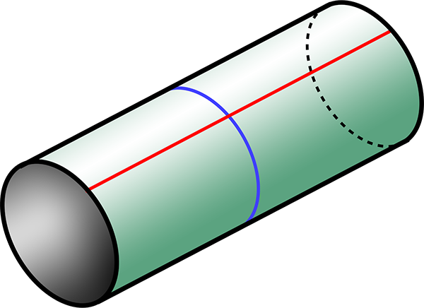
A cylinder, as could be formed by rolling a sheet of paper. The blue line is a line of maximum curvature, wrapped around the cylinder. The red line, along the cylinder perpendicular to the blue line, has zero curvature.

So what surfaces have non-zero Gaussian curvature? By the Theorema Egregium, they must be surfaces that you can’t bend a sheet of paper into without stretching it. An example is the surface of a sphere. If you try to wrap a sheet of paper smoothly around a sphere, you can’t do it without stretching, scrunching, or tearing the paper. If we draw a line around a sphere (like an equator), that’s one principal curvature, equal to 1/r, similar to the cylinder, where r is now the radius of the sphere. A line perpendicular to that (like a line of longitude), also has the same same principal curvature due to the symmetry of the sphere, 1/r. The Gaussian curvature of a sphere is then (1/r)×(1/r) = 1/r².

And then there are surfaces with a saddle shape, bending upwards in one direction and downwards in a perpendicular direction. An example is the surface on the inside of the hole in a torus (or doughnut shape). If you imagine standing on the surface here, in one direction it curves downwards with a radius s equal to that of the solid part of the torus, while in the perpendicular direction the surface curves upwards with radius h, the radius of the hole. Curving upwards is defined as a negative curvature, so the two principal curvatures are 1/s and -1/h, and the Gaussian curvature here is the product, -1/sh.

Torus showing radii

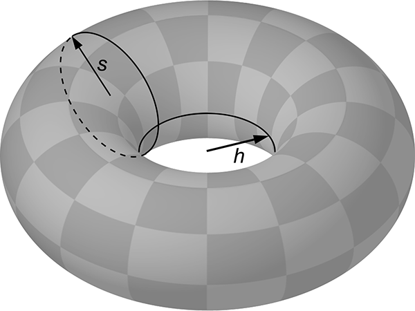
A torus, showing the solid radius s and the radius of the hole h. The point where the two circles intersect has Gaussian curvature -1/sh. (Image modified from public domain image from Wikimedia Commons.)

Here are examples of surfaces with negative, zero, and positive curvature, respectively a hyperboloid, cylinder, and sphere:

Surfaces with negative, zero, and positive curvatures

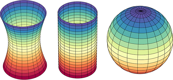
Illustration of surfaces with negative, zero, and positive Gaussian curvature: respectively a hyperboloid, cylinder, and sphere. (Image modified from public domain image from Wikimedia Commons.)

Another way to think about Gaussian curvature is to imagine wrapping a sheet of paper snugly onto the surface. If you can do it without stretching or tearing the paper (such as a cylinder), the curvature is zero. If you have to scrunch the paper up (like wrapping a sphere), the curvature is positive. If you have to stretch/tear the paper (like the saddle or hyperboloid), the curvature is negative. It’s also important to realise that the Gaussian curvature doesn’t need to be the same everywhere – it can vary across the surface. It’s zero at all points on a cylinder, and 1/r² at all points on a sphere, but on a torus the curvature is negative on the inside of the hole and positive on the outside, with lines of zero curvature running around the top and bottom.

Torus showing positive and negative curvatures

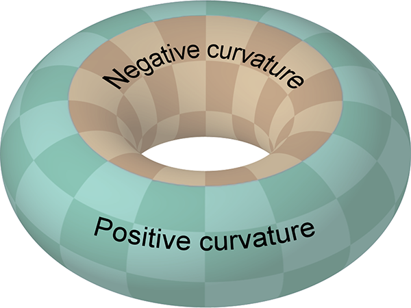
Diagram of a torus, showing regions of positive (green) and negative (orange) Gaussian curvature. The boundary between the regions has zero curvature.

A property of two-dimensional curvature is that it affects the geometry of two-dimensional shapes on the surface. A surface with zero Gaussian curvature we call Euclidean, and the Euclidean geometry matches the familiar geometry we learn at primary and secondary school. This incudes all those properties of circles and triangles and parallel lines that you learnt. In particular, let’s talk about triangles. Triangles have three internal angles and, as we learnt in school, if you add up the sizes of the angles you get 180°. In the angular unit known as radians, 180° is equal to π radians. (To convert from degrees to radians, divide by 180 and multiply by π.)

So, in a Euclidean geometry, the angle sum of a triangle equals π radians. This is the case for triangles drawn on a flat sheet of paper, and it also holds if you wrap the paper around a cylinder. The triangle bends around the cylinder in the positive principal curvature direction, but its Gaussian curvature remains zero (because of the Theorema Egregium). And if you measure the angles and add them up, they still add up to π radians (i.e. 180°).

However if you draw a triangle on a surface of negative curvature, the lines are locally straight but from a three-dimensional point of view they are bowed inwards by the curvature of the surface, pinching the angles to make them smaller.

Saddle shaped surface with triangle

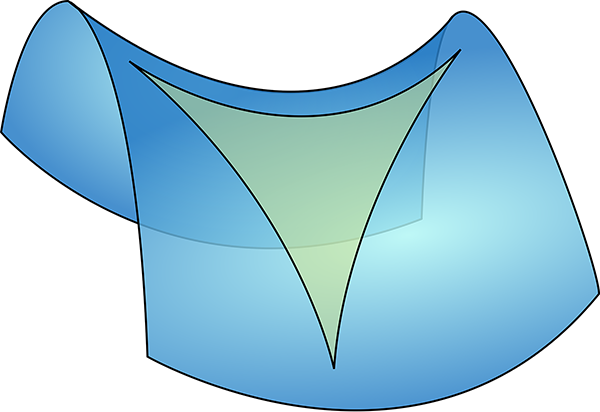
A saddle shaped surface with negative curvature, with a triangle drawn on it. The angles become pinched in and smaller. (Image modified from public domain image from Wikimedia Commons.)

On the other hand, if you draw a triangle on the surface of a sphere, which has positive curvature, the lines seem to bow outwards, making the angles larger.

Spherical shaped surface with triangle

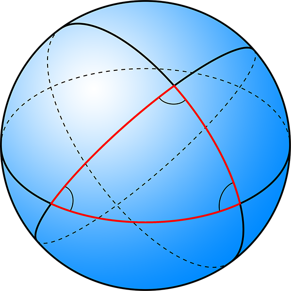
A spherical surface with positive curvature, with a triangle drawn on it. The angles become bulged out and larger. (Image modified from public domain image from Wikimedia Commons.)

Now, here’s the cool thing. On a negative curvature surface, the angle sum of a triangle is less than π radians, while on a positive curvature surface it’s greater than π radians. Imagine a really small triangle on either of these surfaces. Over a very small area, the curvature is not so evident, and the angle sum is only different from π radians by a small amount. But for a larger triangle, the curvature makes a bigger difference, and the angle sum differs from π radians by a larger amount. It turns out there’s a mathematical relationship between the Gaussian curvature of the surface, the size of the triangle, and the amount by which the angle sum differs from π radians:

The angle sum of a triangle = π radians + the integral of the Gaussian curvature over the area of the triangle. [Equation 1]

If you’re not familiar with calculus, the integral part basically means you take small patches of area within the triangle, multiply the Gaussian curvature in the patch by the area of the patch and add them all up. If the Gaussian curvature is constant (such as for a sphere), the integral is just equal to the curvature times the area of the triangle.

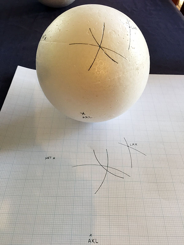
To take a concrete example, imagine a sphere of radius one unit. The surface area of the sphere is 4π square units. Now let’s draw a triangle on the sphere. If we imagine the sphere with lines of latitude and longitude like the Earth, we’ll take the equator as one of our triangle sides, and two lines of longitude running from the North Pole to the equator, 90° apart. The angle between the equator and any line of longitude is 90° (π/2 radians), and the angle at the North Pole between our chosen two lines of longitude is also 90° (by construction). So the angle sum of this triangle is 3π/2 radians, which is π/2 radians greater than π radians.

From equation 1, this means that the integral of the Gaussian curvature over the triangle equals π/2. The area of the triangle is one eighth the surface area of the whole sphere = 4π/8 = π/2 square units. The Gaussian curvature of a sphere is constant, so curvature×(π/2 square units) = π/2, which means the curvature is equal to 1. We said the sphere has a radius of one unit, and Gaussian curvature of a sphere is 1/r², so the curvature is just 1. It all works out!

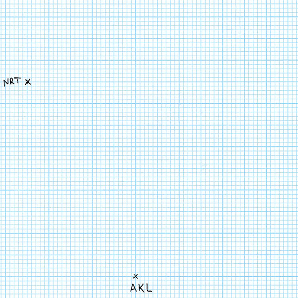
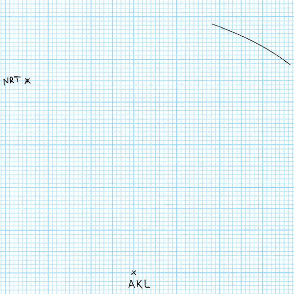
Now imagine we’re looking at such a triangle on the Earth itself. Our edges are the equator, and we’ll take the lines of longitude 30° west (running through eastern Greenland) and 60° east (through Russia and Kazakhstan, among other places). The area of this triangle, if we measured it, turns out to be 63.8 million square kilometres.

A large triangle on Earth

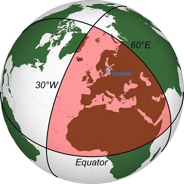
A triangle on Earth, with each angle equal to 90°. (Image modified from public domain image from Wikimedia Commons.)

Applying equation 1:

Angle sum of triangle = π radians + integral of Gaussian curvature over the area of the triangle

3π/2 radians = π radians + Gaussian curvature × 63.8 million square kilometres

π/2 radians = Gaussian curvature × 63.8 million square kilometres

Gaussian curvature = (π/2)/63.8×106

1/r² = (π/2)/63.8×106

r² = 63.8×106/(π/2)

r = √[63.8×106/(π/2)]

r = 6371 kilometres

This is the radius of the Earth. And it’s exactly right. So simply by measuring the angles of a triangle drawn on the surface of the Earth, and the area within that triangle, we can show that the surface of the Earth is not flat, but curved, and we can determine the radius of the Earth.

Obviously I haven’t gone out and measured such a triangle in practice. It would take expensive surveying gear and an extensive travel budget, but in principle you can certainly do it. Because the effect of the curvature depends on the size of the triangle, you need to survey a large enough area to detect the Earth’s curvature. How large?

I did some searching for angular accuracy of large scale surveys, but didn’t find anything particularly convincing. As a first estimate, I guessed conservatively that you might be able to measure the angles of a very large triangle to an accuracy of a tenth of a degree. With three corners, this makes the necessary deviation of the angle sum from π equal to 0.005 radians. The necessary area to see the effect of curvature is this number times the square of Earth’s radius, which gives 203,000 square kilometres, about the area of Belarus, or Kyrgyzstan. If you surveyed a triangle that big, measuring the area accurately and the angles to within 0.1° accuracy, you could experimentally verify that the Earth was curved, not flat.

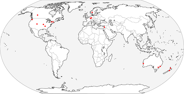
A reference on the accuracy of Global Navigation Satellite Systems used for geodetic surveying [1], gives an angular accuracy better than my guess, in the order of 2 minutes of arc (i.e. 1/30°) for this method. This gives us a necessary area of 20,300 square kilometres, about the area of Slovenia or Israel. Another reference on laser scanners used in surveying [2] gives an angular resolution of 3 mm over a range of 100 m, equivalent to 6 seconds of arc. If we can survey the angles of a triangle this accurately, we only need to measure an area of 1220 square kilometres, which is smaller than the Indian Ocean island nation of Comoros, and about the size of Gotland, Sweden’s largest island (circled in blue in the above figure).

Interestingly, Gauss was likely inspired to develop a mathematical treatment of curvature by his experience as a surveyor. In the 1820s, he was tasked with surveying the Kingdom of Hanover (now part of Germany). To check the calibration of his equipment, he surveyed a large triangle with corners on the tops of the mountains Brocken, Hoher Hagen, and Großer Inselsberg, encompassing an area of 3000 km². Each mountaintop had direct line of sight to the others, so this was not actually a survey of a curved triangle along the surface of the Earth, but rather a flat triangle through 3D space above the surface of the Earth. Gauss considered this a validation check on the accuracy of the equipment, rather than a test to see if the Earth was curved. He measured the angles and added them up, finding the sum to be 180° to within his measurement uncertainty. Although this was not the curvature experiment described above, Gauss later drew on his surveying experience to investigate the properties of curved surfaces.

This concludes the “Earth is a Globe” portion of this entry, but there are two other cool applications of differential geometry:

Firstly, curvature of this type applies not only to two-dimensional surfaces, but also to three-dimensional space. It’s possible that the 3D space we live in has a non-zero curvature. This sort of curvature is tied up in general relativity, gravity, and the expansion of the universe. We know the curvature of space is very close to zero, but not if it’s exactly zero – it may be slightly positive or negative. To measure the curvature of space directly, all we need to do is measure the angles of a large enough triangle. In this case, large enough means millions of light years. We can’t send surveyors out that far, but imagine if we contacted two alien civilisations by radio. It would take millions of years to coordinate, but we could ask them to measure the angles between our sun and the sun of the other civilisation at some predetermined time, and we could combine it with our own measurement, to determine the angle sum of this enormous triangle. If it doesn’t equal π radians, we’d have a direct measurement of the curvature of the universe.

Secondly, and perhaps more practically, the Theorema Egregium helps us eat pizza. If you take a long slice of pizza (and the base is not thick/crispy enough to be rigid), the tip can flop down messily.

A floppy slice of pizza

A slice of pizza flopping along its length. Danger of making a mess!

Differential geometry to the rescue! The slice begins flat, so has zero Gaussian curvature. It can bend in one direction, flopping down and making a mess. But if we fold the slice by pushing the ends of the crust upwards and together, this creates a non-zero principal curvature across the slice. By the Theorema Egregium, the Gaussian curvature (the product of the principal curvatures) must remain zero, so the principal curvature in the perpendicular direction along the slice is now fixed at zero, and the slice cannot flop down any more!

A rigid slice of pizza

A slice of pizza curved perpendicular to the length can no longer flop. Danger averted, thanks to differential geometry!

References:

[1] Correa-Muños, N. A., Cerón-Calderón, L. A. 2018. “Precision and accuracy of the static GNSS method for surveying networks used in Civil Engineering”. Ingeniería e Investigación, 38(1), p. 52-59, 2018. https://doi.org/10.15446/ing.investig.v38n1.64543

[2] Fröhlich, C. Mettenleiter, M. “Terrestrial laser scanning—new perspectives in 3D surveying”. International archives of photogrammetry, remote sensing and spatial information sciences, 36(8), p.W2, 2004. https://www.semanticscholar.org/paper/TERRESTRIAL-LASER-SCANNING-–-NEW-PERSPECTIVES-IN-3-Froehlich-Mettenleiter/4e117d837e43da8b9e281aec1ce9a8625430b6c3

16. Lunar eclipses

Lunar eclipses occur when the Earth is positioned between the sun and the moon, so that the Earth blocks some or all of the sunlight from directly reaching the moon. Because of the relative sizes of the sun, Earth, and moon, and their distances from one another, the Earth’s shadow is large enough to completely cover the moon.

To talk about eclipses, we need to define some terms. The sun is a large, extended source of light, not a point source, so the shadows that objects cast in sunlight have two components: the umbra, where light from the sun is totally blocked, and the penumbra, where light from the sun is partially blocked.

Diagram showing the umbra and penumbra cast by the Earth. Not to scale. Public domain image from Wikimedia Commons.

When the moon passes entirely inside the Earth’s umbra, that is a total lunar eclipse. Although no sunlight reaches the moon directly, the moon is not completely dark, because some sunlight refracts (bends) through the Earth’s atmosphere and reaches the moon. This light is red for the same reason that sunsets on Earth tend to be red: the atmosphere scatters blue light more easily than red, so red light penetrates large distances of air more easily. This is why during a total lunar eclipse the moon is a reddish colour. Although a totally eclipsed moon looks bright enough to our eyes, it’s actually very dark compared to a normal full moon. Our eyes are very good at compensating for the different light levels without us being aware of it.

Total lunar eclipse of 28 August 2007 (photographed by me). 1 second exposure at ISO 800 and aperture f/2.8.

The amount of refracted light reaching the moon depends on the cleanliness of the Earth’s atmosphere. If there have been recent major volcanic eruptions, then significantly less light passes through to reach the moon. The brightness of the moon during a total lunar eclipse can be measured using the Danjon scale, ranging from 0 for very dark eclipses, to 4 for the brightest ones. After the eruption of Mount Pinatubo in the Philippines in 1991, the next few lunar eclipses were extremely dark, with the eclipse of December 1992 rating a 0 on the Danjon scale.

When the moon is only partly inside the Earth’s umbra, that is a partial lunar eclipse. A partial phase occurs on either side of a total lunar eclipse, as the moon passes through the Earth’s shadow, and it can also occur as the maximal phase of an eclipse if the moon’s orbit isn’t aligned to carry it fully within the umbra. During a partial eclipse phase, you can see the edge of the Earth’s umbral shadow on the moon.

Partial phase of the same lunar eclipse of 28 August 2007. 1/60 second exposure at ISO 100 and f/8, which is 1/3840 the exposure of the totality photo above. If this photo was 3840 times as bright, the dark part at the bottom would look as bright as the totality photo (and the bright part would be completely washed out).

Lunar eclipses can only occur at the full moon – those times when the sun and moon are on opposite sides of the Earth. The moon orbits the Earth roughly once every 29.5 days and so full moons occur every 29.5 days. However, lunar eclipses occur only two to five times per year, because the moon’s orbit is tilted by 5.1° relative to the plane of the Earth’s orbit around the sun. This means that sometimes when the moon is full it is above or below the Earth’s shadow, rather than inside it.

Okay, so what can lunar eclipses tell us about the shape of the Earth? A lunar eclipse is a unique opportunity to see the shape of the Earth via its shadow. A shadow is the same shape as a cross-section of the object casting the shadow. Let’s have another look at the shape of Earth’s shadow on the moon, in a series of photos taken during a lunar eclipse:

Montage of photos taken over 83 minutes during the lunar eclipse of 28 August 2007. Again, the bottom row of photos have 3840 times the exposure of the top row, so the eclipsed moon is nearly 4000 times dimmer than the full moon.

As you can see, the edge of the Earth’s shadow is curved. The fact that the moon’s surface is curved doesn’t affect this, because we are looking from the same direction as the Earth, so we see the same cross-section of the moon. (Your own shadow looks the shape of a person to you, even if it falls on an irregular surface where it looks distorted to someone else.) So from this observation we can conclude that the edge of the Earth is rounded.

Many shapes can cause a rounded shadow. However, if you observe multiple lunar eclipses, you will see that the Earth’s shadow is always round, and what’s more, it always has the same radius of curvature. And different lunar eclipses occur at any given location on Earth with the moon at different points in the sky, including sometimes when the moon is not in the sky (because the location is facing away from the moon). This means that different lunar eclipses occur when different parts of the Earth are facing the moon, which means that different parts of the Earth’s edge are casting the shadow edge on the moon. So from these observation, we can see that the shape of the shadow does not depend on the orientation of the Earth to the moon.

There is only one solid shape for which the shape of its shadow doesn’t depend on the object’s orientation. A sphere. So observations of lunar eclipses show that the Earth is a globe.

Addendum: A common rebuttal by Flat Earthers is that lunar eclipses are not caused by the Earth’s shadow, but by some other mechanism entirely – usually another celestial object getting between the sun and moon and blocking the light. But any such object is apparently the same colour as the sky, making it mysteriously otherwise completely undetectable, and does not have the simple elegance of explanation (and the supporting evidence from numerous other observations) of the moon moving around the Earth and entering its shadow.

15. Trilateration

Trilateration is the method of locating points in space based on measuring the distances from known reference locations. It is used in surveying and navigation, similarly to the related method of triangulation, which technically uses the measurement of angles, not distances. For this entry we’re going to get practical and attempt to do some trilateration, using distances between some major cities in the world. To do this, I’ll need some equipment:

Equipment used

I acquired graph paper, a ruler, a tape measure, a pen, a pair of compasses, and a couple of large polystyrene balls.

I began my first scale drawing on a piece of graph paper. I’ve picked Auckland, New Zealand, as one of my cities of interest. Since nothing is on the paper yet, I can place Auckland wherever I want to. So I draw a cross indicating the position of Auckland and label it AKL (the city’s international airport code).

Auckland's position

For my second city, I’ve chosen Tokyo, Japan. According to a flight distance reference website, the travelling distance between Auckland and Tokyo, or more specifically between Auckland Airport and Tokyo’s Narita Airport, is 8806 kilometres. My graph paper has 2 mm squares, and (for reasons that will become clear in a minute) I’m using a scale of 86.1 km/mm. So I take a pair of compasses and set the distance from the metal point to the pen tip to be 102.3 mm as best I can. That’s 51 and a bit grid squares. I place the point in the centre of the AKL cross and mark a point on the paper 102.3 mm away with the pen tip. I enlarge the point to a cross and label it NRT (for Narita Airport). It doesn’t matter which direction I choose to place Tokyo from Auckland, because at this point there are no other constraints.

Tokyo's position

For my third city, I choose Los Angeles, USA. Los Angeles Airport, LAX, is 10467 km from Auckland, and 8773 km from Tokyo Narita. To locate LAX on my scale drawing, I first set my compasses with a distance of 10467 / 86.1 = 121.6 mm. With this distance setting, I draw an arc centred on AKL.

Los Angeles' position from Auckland

All of the points on this arc are the correct distance from Auckland to be Los Angeles. But we have another constraint – Los Angeles also has to be the correct distance from Tokyo. So I set my compasses to 8773 / 86.1 = 101.9 mm, and draw an arc centred at NRT.

Los Angeles' position nailed down

The intersection of these two arcs is the point that is both the correct scale distance from Auckland and Tokyo, so I label the intersection point LAX. So far, so good. We have three world cities with their relative positions accurately plotted to scale. Let’s add a fourth city! For the fourth city, I’ll choose something somewhere in the middle of the first three: Honolulu, USA. For starters, Honolulu is 7063 km from Auckland. So I draw an arc with radius 7063 / 86.1 = 82.0 mm centred on AKL.

Honolulu's position from Auckland

Honolulu is 6146 km from Tokyo. So I draw an arc with radius 6146 / 86.1 = 71.4 mm centred on NRT.

Honolulu's position from Auckland and Tokyo

Now in theory this is enough to give us the location of Honululu. It must be on both the arc centred at Auckland and on the arc centred at Tokyo – so it has to be at the intersection of those two arcs. But wait! We have more information than that. We also know that Honolulu is 4113 km from Los Angeles. So I draw an arc with radius 4113 / 86.1 = 47.8 mm centred on LAX.

Honolulu's position from Auckland, Tokyo, and Los Angeles

For the flight distances to be correct, Honolulu Airport (HNL) must be on all three arcs that I’ve drawn. But the arcs don’t all intersect at the same point. So where is Honolulu? According to the rules of geometry, anywhere we put it results in at least one of the distances being wrong. In the worst case, the the AKL-LAX intersection is 10 mm on the drawing from the NRT-LAX intersection, an error of 861 kilometres, which is 300 km longer than the entire chain of populated Hawaiian Islands from Niihau to Hawaii. Obviously a navigation error this large when trying to find Honolulu in the midst of the Pacific Ocean would be disastrous.

What’s gone wrong? Well, I’ve attempted to draw these distances to scale on a flat piece of paper. The error shows the distortion caused by trying to map the shape of the Earth onto a flat surface. The distances are all correct, but in reality they don’t lie in the same plane. So let’s try another approach. I’m going to map the distances onto a scale model of the Earth as a sphere.

To do this, I got a polystyrene sphere from an art supply shop. I measured the circumference using a tape measure to be 465 mm. Dividing the average circumference of the Earth by this gives me a scale of 86.1 km/mm (which is where I got the scale that I used for the drawing above). Now I just need to repeat the steps above, but plot the points and arcs on the surface of the sphere. But there’s one small wrinkle: flight distances are measured along the surface of the Earth, but the compasses step off the distance in a straight line, as measured through the Earth. To get the correct scale distance to set the compasses, we need to do a little geometry:

Geometry figure: surface distance versus straight line distance

The distance along the surface of the Earth is d, the distance through the Earth is x, and the radius of the Earth is r. In radians, the angle θ is d/r. Now according to the cosine rule of trigonometry:

x² = r² + r² – 2r² cos θ

x² = 2r²(1 – cos(d/r))

So plugging in d and r we can find the distance x to set the compasses to (at the correct scale). Here’s a summary table:

Cities	Distance (km)	Scale distance (mm)	Compasses distance (mm)
AKL-NRT	8806	102.3	94.3
AKL-LAX	10467	121.6	108.4
NRT-LAX	8773	102.0	94.0
AKL-HNL	7063	82.1	77.9
NRT-HNL	6146	71.4	68.6
LAX-HNL	4113	47.8	46.9

Using the distances in the Compasses column on my polystyrene sphere, and following the same steps as above for the graph paper, produced this:

Honolulu's position on a sphere

The arcs drawn with the correct scale distances of Honolulu from Auckland, Tokyo, and Los Angeles all intersect at exactly the same point on the surface of the sphere. We’ve found Honolulu!

So by experiment, trilateration of points on the Earth’s surface does not work if you use a flat surface to map the points. It only works if you use a sphere.

Addendum: I bought two spheres because I was prepared for the first attempt to be a little bit out due to any small inaccuracies or mistakes in my setting the correct compasses distances. But as it turned out I only needed the one. I was pleasantly surprised when it worked so well the first time.

12. The sun

Possibly the most obvious property of our sun is that it is visible from Earth during daylight hours, but not at night. The visibility of the sun is in fact what defines “day time” and “night time”. At any given time, the half of the Earth facing the sun has daylight, while the other half is in the shadow of the Earth itself, blocking the sun from view. It’s trivial to verify that parts of the Earth are in daylight at the same time as other parts are in night, by communicating with people around the world.

The first physical property of the sun to be measured was how far away it is. In the 3rd century BC, the ancient Greek Aristarchus of Samos (who we met briefly in 2. Eratosthenes’ measurement) developed a method to measure the distance to the sun in terms of the size of the Earth, using the geometry of the relative positions of the sun and moon. Firstly, when the moon appears exactly half-illuminated from a point on Earth, it means that the angle formed by the sun-moon-Earth is 90°. If you observe the angle between the sun and the moon at this time, you can determine the distance to the sun as a multiple of the distance to the moon.

Aristarchus's method 1

Geometry of the sun, moon, and Earth when the moon appears half-illuminated.

In the figure, if you measure the angle θ, then the ratio of the distance to the sun S divided by the distance to the moon M is the reciprocal of the cosine of θ. Aristarchus then used the size of the shadow of Earth on the moon during a lunar eclipse to obtain further equations relating the distances to the sun and moon and the size of the Earth.

A medieval copy of Aristarchus’s drawing of the geometry of the sun-Earth-moon system during a lunar eclipse. (Public domain image.)

By combining these results, you can calculate the distances to both the sun and the moon in terms of the radius of the Earth. Aristarchus got the wrong answer, estimating that the sun was only about 19 times further away than the moon, because of the limited precision of his naked eye angle measurements (it’s actually 390 times further away). But Eratosthenes later made more accurate measurements (which were again discussed in Eratosthenes’ measurement), most likely using the same method.

The first rigorous measurement of the absolute distance to the sun was made by Giovanni Cassini in 1672. By this time, observations of all the known celestial bodies in our solar system and some geometry had well and truly established the relative distances of all the orbits. For example, it was known that the orbital radius of Venus was 0.72 times that of Earth, while the orbit of Mars was 1.52 times that of Earth. To measure the absolute distance to the sun, Cassini used a two-step method, the first step of which was measuring the distance to the planet Mars. This is actually a lot easier to do than measuring the distance to the sun, because Mars can be seen at night, against the background of the stars.

Cassini dispatched his colleague Jean Richer to Cayenne in French Guiana, South America, and the two of them arranged to make observations of Mars from there and Paris at the same time. By measuring the angles between Mars and nearby stars, they determined the parallax angle subtended by Mars across the distance between Paris and Cayenne. Simple geometry than gave the distance to Mars in conventional distance units. Then applying this to the relative distances to Mars and the sun gave the absolute distance from the Earth to the sun.

Since 1961, we’ve had a much more direct means of measuring solar system distances. By bouncing radar beams off the moon, Venus, or Mars and measuring the time taken for the signal to return at the speed of light, we can measure the distances to these bodies to high precision (a few hundred metres, although the distances to the planets change rapidly because of orbital motions) [1].

The Earth orbits the sun at a distance of approximately 150 million kilometres. Once we know this, we can work out the size of the sun. The angular size of the sun as seen from Earth can be measured accurately, and is 0.53°. Doing the mathematics, 0.53°×(π/180°)×150 = 1.4, so the sun is about 1.4 million kilometres in diameter, some 109 times the diameter of the Earth. This is the diameter of the visible surface – the sun has a vast “atmosphere” that we cannot see in visible light. Because of its vast distance compared to the size of the Earth, the sun’s angular size does not change appreciably as seen from different parts of the Earth. The difference in angular size between the sun directly overhead and on the horizon (roughly the Earth’s radius, 6370 km, further away) is only about 6370/150000000×(180°/π) = 0.002°.

Our sun is, in fact, a star – a huge sphere composed mostly of hydrogen and helium. It produces energy from mass through well-understood processes of nuclear fusion, and conforms to the observed properties of stars of similar size. The sun appears much larger and brighter than stars, and heats the Earth a lot more than stars, because the other stars are all so much further away.

Our sun, observed in the ultraviolet as a false colour image by NASA’s Solar Dynamics Observatory satellite. (Public domain image by NASA.)

Like all normal stars, the sun radiates energy uniformly in all directions. This is expected from the models of its structure, and can be inferred from the uniformity of illumination across its visible disc. The fact that the sun’s polar regions are just as bright as the equatorial edges implies that the radiation we see in the ecliptic plane (the plane of Earth’s orbit) is reproduced in all directions out of the plane as well.

NASA’s Ulysses solar observation spacecraft was launched in 1990 and used a gravity slingshot assist from Jupiter to put it into a solar orbit inclined at about 80° to the ecliptic plane. This allowed it to directly observe the sun’s polar regions.

Polar orbit of Ulysses around the sun, giving it views of both the sun’s north and south poles. (Public Domain image by NASA.)

Now, I tried to find scientific papers using data from Ulysses to confirm that the sun indeed radiates electromagnetic energy (visible light, ultraviolet, etc.) uniformly in all directions. However, it seems that no researchers were willing to dedicate space in a paper to discussing whether the sun radiates in all directions or not. It’s a bit like looking for a research paper that provides data on whether apples fall to the ground or not. What I did find are papers that use data from Ulysses’ solar wind particle flux detectors to measure if the energy emitted by the sun as high energy particles varies with direction.

Solar proton flux versus latitude

Proton flux density observed by Ulysses at various heliographic (sun-centred) latitudes. -90 is directly south of the sun, 0 would be in the ecliptic plane. The track shows Ulysses’ orbit, changing in distance and latitude as it passes under the sun’s south polar regions. Figure reproduced from [2].

Solar wind energy flux versus latitude

Various solar wind plasma component energy fluxes observed by Ulysses at various heliographic latitudes. Figure reproduced from [3].

As these figures show, the energy emitted by the sun as solar wind particles is pretty constant in all directions, from equatorial to polar. Interestingly, there is a variation in the solar wind energy flux with latitude: the solar wind is slower and less energetic close to the plane of the ecliptic than at higher latitudes. The solar wind, unlike the electromagnetic radiation from the sun, is affected by the structure of the interplanetary medium. The denser interplanetary medium in the plane of the ecliptic slows the wind. The amount of slowing provides important constraints on the physics of how the solar wind particles are accelerated in the first place.

Anyway, given there are papers on the variation of solar wind with direction, you can bet your bottom dollar that there would be hundreds of papers about the variation of electromagnetic radiation with direction, if it had been observed, because it goes completely counter to our understanding of how the sun works. The fact that the sun radiates uniformly in all directions is such a straightforward consequence of our knowledge of physics that it’s not even worth writing a paper confirming it.

Now, in our spherical Earth model, all of the above observations are both consistent and easily explicable. In a Flat Earth model, however, these observations are less easily explained.

Why is the sun visible in the sky from part of the Earth (during daylight hours), while in other parts of the Earth at the same time it is not visible (and is night time)?

The most frequently proposed solution for this is that the sun moves in a circular path above the disc of the Flat Earth, shining downwards with a sort of spotlight effect, so that it only illuminates part of the disc. Although there is a straight line view from areas of night towards the position of the sun in the sky, the sun does not shine in that direction.

Given that we know the sun radiates uniformly in all directions, we know this cannot be so. Furthermore, if the sun were a directional spotlight, how would such a thing even come to be? Directional light sources do occur in nature. They are produced by synchrotron radiation from a rapidly rotating object: for example, a pulsar. But pulsars rotate and sweep their directional beams through space on a timescale of approximately one second. If our sun were producing synchrotron radiation, its spotlight beam would be oscillating many times per minute – something which is not observed.

Even furthermore, if the sun is directional and always above the plane of the Flat Earth, it should be visible in the night sky, as an obscuration passing in front of the stars. This prediction of the Flat Earth model is not seen – it is easy to show that no object the size of the sun obscures any stars at night.

And yet furthermore, if the sun is directional, there are substantial difficulties in having it illuminate the moon. Some Flat Earth models acknowledge this and posit that the moon is self-luminous, and changes in phase are caused by the moon itself, not reflection of sunlight. This can easily be observed not to be the case, since (a) there are dark shadows on the moon caused by the light coming from the location of the sun in space, and (b) the moon darkens dramatically during lunar eclipses, when it is not illuminated by the sun.

In addition to the directional spotlight effect, typical Flat Earth models state that the distance to the sun is significantly less than 150 million kilometres. Flat Earth proponent Wilbur Glenn Voliva used geometry to calculate that the sun must be approximately 3000 miles above the surface of the Earth to reproduce the zenith angles of the sun seen in the sky from the equator and latitudes 45° north and south.

Voliva's distance to the sun calculation

Wilbur Glenn Voliva’s calculation that the sun is 3000 miles above the Flat Earth. Reproduced from Modern Mechanics, October 1931, p. 73.

Aside from the fact that Voliva’s distance does not give the correct zenith angles for any other latitudes, it also implies that the sun is only about 32 miles in diameter, given the angular size seen when it is overhead, and that the angular size of the sun should vary significantly, becoming only 0.53°/sqrt(2) = 0.37° when at a zenith angle of 45°. If the sun is this small, there are no known mechanisms than can supply the energy output it produces. And the prediction that the sun would change in angular size is easily disproved by observation.

The simplest and most consistent way of explaining the physical properties of our sun is in a model in which the Earth is a globe.

References:

[1] Muhleman, D. O., Holdridge, D. B., Block, N. “The astronomical unit determined by radar reflections from Venus”. The Astrophysical Journal, 67, p. 191-203, 1962. https://doi.org/10.1086/108693

[2] Barnes, A., Gazis, P. R., Phillips, J. L. “Constraints on solar wind acceleration mechanisms from Ulysses plasma observations: The first polar pass”. Geophysical Research Letters, 22, p. 3309-3311, 1995. https://doi.org/10.1029/95GL03532

[3] Phillips, J. L., Bame, S. J., Barnes, A., Barraclough, B. L., Feldman, W. C., Goldstein, B. E., Gosling, J. T., Hoogeveen, G. W., McComas, D. J., Neugebauer, M., Suess, S. T. “Ulysses solar wind plasma observations from pole to pole”. Geophysical Research Letters, 22, p. 3301-3304, 1995. https://doi.org/10.1029/95GL03094

2.c Eratosthenes and the Flat Earth model

A reader has pointed out that we can also use the data collected in our Eratosthenes experiment to test the hypothesis that the Earth is flat and that the difference in shadows is caused by the sun being a relatively small distance from the flat Earth. And we can compare this test to a test of our round Earth hypothesis.

If the Earth is flat, and we make an observation like Eratosthenes, that a vertical stick in one location casts no shadow, while a vertical stick some distance north (or south) does cast a shadow, then we can use geometry to figure out how far away the sun must be.

Distance to the sun in a flat Earth model

Using similar triangles to determine the distance from a flat Earth to the sun, given an observation of the shadow of a vertical stick, and knowing the distance from a point where the sun is overhead.

If the Earth is indeed flat then when we do this calculation for each of our 19 observations we should get the same answer, to within any experimental error. In particular, there should be no systematic difference in our answers that depends on the distance from the equator. Analogously, in our round Earth model, the circumference we have calculated for the Earth from each of our observations should also be the same to within experimental errors, and show no systematic difference depending on distance from the equator.

So let’s test those things! Here are graphs of the results, on which I’ve included a linear least squares best fit line, showing the line’s equation and statistical R² score. The R² value, or coefficient of determination, is a measure of how likely the data values (the circumference of the Earth in the round Earth hypothesis, or the distance to the sun in the flat Earth hypothesis) are to be correlated with the fixed values (the distance from the equator in both cases). We’ll discuss that after we see the data.

Earth's circumference versus distance from equator

Plot of 19 measurements of the Earth’s circumference, assuming the round Earth model, versus distance from the equator.

Distance to sun versus distance from equator

Plot of 19 measurements of the distance of the sun from Earth, assuming the flat Earth model, versus distance from the equator.

The first thing to notice is that in the top plot, the circumference of the Earth values look fairly evenly scattered around the true value. In the bottom plot, the calculated values for the distance of the sun from Earth are not evenly scattered; they show a pretty clear trend of giving larger distances for the data points closer to the equator and smaller distances for data points further from the equator. We can quantify this by looking at the straight line fits to the data and in particular the R² value.

To do a rigorous statistical test, we need to set up our two possible null hypotheses. These are statements that for the purpose of our statistical test we assume are true, and then we calculate the probability that what we observe could happen by random chance. Our two null hypotheses are:

1. For the spherical Earth model, the calculated circumference of Earth is independent of the distance from the equator of our data points.

2. For the flat Earth model, the calculated distance of the sun from Earth is independent of the distance from the equator of our data points.

To test these, we use a probability distribution that tells us how likely our observed R² scores are. An appropriate one to use is Student’s t-distribution. We calculate Student’s t-distribution function for 19 data points and 2 degrees of freedom (the y-intercept and the slope of our fitted line), determine a value for the function below which 95% of the probability distribution lies, and convert this to an R² value using the known transformation. In simpler terms (TL;DR), we’re working out a number R²(P<0.05) which, if our calculated values are independent of distance from the equator, then we would expect 95% of experiments to give an R² value less than the number R²(P<0.05).

Doing the maths, our value for R²(P<0.05) is 0.334. What this means is that if our R² value is greater than 0.334, then we should reject our null hypothesis – the data are statistically inconsistent with the hypothesis (at the 95% confidence level, for those who like statistical rigour*). On the other hand, if our R² value is less than 0.334, we cannot reject our null hypothesis – we haven’t proven it to be true, we have just shown that our data are consistent with it.

Now let’s look at our calculated R² values. For the spherical Earth hypothesis, R² = 0.1358. This is less than the critical value, so our data are consistent with our hypothesis. In contrast, for the flat Earth model, R² = 0.9162. This is greater than the critical value, so we can confidently reject the flat Earth hypothesis as inconsistent with our experiment!

So there you have it. Not only did we successfully measure the circumference of the Earth to within our experimental errors, we have now also shown that our experimental results are consistent with a spherical Earth model, and inconsistent with a flat Earth model.

* Note: Choosing the 95% confidence level is typical for statistical hypothesis testing. You should always choose your confidence level before performing the calculations, to avoid any bias in your reporting. You can choose other levels, such as 99%. If I’d done that, we would have found that our data are also inconsistent with the flat Earth model at the more stringent 99% confidence level. In fact, calculating backwards, the confidence level of our rejection is a bit above 99.7%.

2.b Eratosthenes’ measurement results

Thank you to everyone who participated in our measurement of the Earth using Eratosthenes’ method! And thank you to those who tried but were frustrated by the weather – I received several reports of bad weather from the UK, France, and parts of the USA. But we have collected 19 successful observations, from 7 countries: New Zealand, Australia, Israel, Germany, Norway, USA, and Canada. I’ve plotted the locations of the observations on the following map.

Map of measurement locations

Map of observation locations. 16 locations are plotted; 3 of the 19 measurements were taken in the same city as another measurement.

The reason we did this experiment on the date of the equinox (20/21 March) is because that is when the sun is directly over the equator. Rather than use ancient Syene in Egypt as our reference point, where the sun is directly overhead on the summer solstice, we’re doing our calculations based on distance from the equator.

Ideally, I’d have asked all of you to measure the length of your vertical stick, the length of its shadow, and the distance you are away from the nearest point where your stick cast no shadow (which would be on the equator either due south or north of your location). Although in principle you can measure your distance from this point by travelling due south or north to the equator and keeping an accurate log of distance travelled, this would almost certainly have lowered the participation numbers! So as a proxy, I asked for your locations – either the city, or an accurate reading of your latitude from a GPS unit or Google Maps or something similar. This is really just a shortcut so that I can calculate your distance from the equator. And yes, although the existence of “degrees of latitude” is based on the premise that the Earth is spherical, the simple multiplicative relationship between distance and the numbers we call “latitude” still holds in the real world (even if the Earth is flat).

Some summary statistics:

Number of data points: 19
Shortest distance from equator: 3196 km (Geraldton, Australia)
Longest distance from equator: 6662 km (Oslo, Norway)
Shortest stick used: 31.5 cm
Longest stick used: 250.2 cm

The calculations proceeded as follows:

1. For each location, I calculated the distance from the equator, using the provided latitude.

2. I calculated the angle of the stick’s shadow from the vertical: shadow angle = arctangent(shadow length / stick length).

3. I calculated the circumference of the Earth for each measurement: circumference = 4 × distance from equator × 90°/(shadow angle). Here is a graph of the resulting 19 measurements of the Earth’s circumference, plotted against the length of the stick used in each case.

Map of measurement locations

Plot of 19 measurements of the Earth’s circumference, versus shadow stick length. As the sticks get longer, the results tend to get more accurate, because it is easier to measure the length of the shadow to a smaller percentage error.

4. I calculated the average of the 19 different measurements of circumference, as well as the standard error of the mean, a statistical measure of the expected uncertainty in the average value. (In experiments like this, where we take multiple independent measurements of the same value, we expect there to be some random errors in each result, caused by slight inaccuracies in measuring the lengths of the sticks and shadows. Our best overall estimate is the average of the results, and the amount of scatter in the results can be used to estimate the likely size of any error in the average.)

The result we achieved is that we measured the circumference of the Earth to be 39926 km, with a standard error of 163 km, or (39926 ± 163) km. What this means is that statistically we expect the true value to lie somewhere between 39763 km and 40089 km.

The polar circumference of the Earth is in fact 40008 km, which lies neatly within this range. So we did it! We measured the circumference of the Earth, and we got the right answer to within the statistical uncertainty of our method!

In one small wrinkle, when everyone was reporting their measurements to me, one person reported that his measurement might be a little bit wrong, because he didn’t have access to a level or any other means of ensuring that his stick was exactly vertical when he took the measurement. So he was unsure whether his data should really be included or not. As it turns out, his data produced the measurement with the largest error, the lowest data point on the graph. If we remove his measurement, our average and standard error become: (40012 ± 147) km. Our average is now even closer to the correct answer, a mere 4 km different. If we made many more measurements, being careful to minimise our random errors, we could expect our result to be even better.

So thank you again to all who participated. Now you can honestly brag that you have measured the size of the Earth!

2.a Making Eratosthenes’ measurement

Performing the experiment described in 2. Eratosthenes’ measurement.

The equinox here in Sydney occurred on 21 March, with local noon at 13:02 local time. Unfortunately the day dawned grey and rainy, with bands of heavy rain blowing in from the south.

As midday drew closer the rain eased off tantalisingly, and there was even a glimpse of blue sky, only to be followed by more heavy rain. Undaunted, a friend joined me for an expedition to a suitable location to make the measurement. I took with me my handy wizard staff to serve as the vertical stick, and a spirit level and tape measure.

We found some flat ground near the McMahons Point ferry wharf, and waited for a break in the clouds. My friend suggested that if we encountered any police and they asked why we were carrying around a quarterstaff, we should say, “Ohhh, just doing a little weather experiment”.

Waiting for the clouds to clear

Waiting for the clouds to clear.

Magically, about 15 minutes before solar noon, the clouds parted and a hot sun shone down out of the sky. We took some quick measurements in case the patchy clouds obscured the sun at the critical time, and they drifted across the sun, turning it on and off as we waited.

Fortunately, around 13:02, there was a good few minutes of uninterrupted sunshine and we measured the shadow of the staff carefully a few times, making sure the staff was held vertical with the spirit level.

Sunshine at local solar noon

Sunshine at local solar noon. Boldly doing Science!

Science successfully done, we headed to a nearby Japanese restaurant for a well-earned lunch!

I’ve been receiving measurements from all across the world today, and have run some preliminary numbers to get results. They look pretty good! But I’ll wait until everyone’s measurements are in before presenting a full report.

5. Horizon dip angle

[audio version of this article]

We’re all familiar with the horizon. Informally, the horizon is as far as you can see, where the sky apparently meets the ground. The horizon of the Earth will come up in several of the proofs we’ll be looking at, but today we’ll be looking at one specific property of the horizon.

Firstly, we need to define our terms more precisely, and recognise that there are three different types of horizon. For the first type, the horizon is defined by a plane perpendicular to the direction of up and down. Up and down are defined by the direction of gravity. If we’re standing on the surface of Earth, then the force of gravity has a specific direction, which we call down. Now look exactly perpendicular to this direction. You can spin on the spot, looking perpendicular to the down direction at all times. This defines a horizontal plane; indeed the very word “horizontal” is derived from “horizon”. This horizon you are looking at is called the astronomical horizon. It might also sensibly be called the geometric or mathematical horizon.

Now let’s define the horizon in a different way. Imagine standing on the surface of the Earth, in a relatively flat area such as an open plain, or perhaps looking out to sea. Look in the direction of the apparent line where the sky meets the Earth’s surface. This is what most people usually think of when they think of “the horizon”, and this is called the true horizon.

A third type of horizon occurs when you’re standing in a place where the landscape is not particularly flat. The true horizon might be obscured by mountains or trees or buildings or whatever. In this case, as far as you can see is called the visible horizon. If the visible horizon obscures the true horizon, then the obstructions need to be projecting above the notionally smooth surface of the Earth, so the visible horizon must be higher and closer than the true horizon (or at the same place as the true horizon if there are no obstructions).

Horizon definitions

The three types of horizon.

Let’s think about the case where there are minimal obstructions and the visible horizon is more or less the same as the true horizon. Now the question arises: Is the true horizon the same as the astronomical horizon, or different?

If the Earth is flat, the astronomical horizon is a plane parallel to the (flat) ground, at the height of the human observer’s eyes. The true horizon is the plane of the Earth itself. These two planes run parallel and, by the laws of perspective, appear to converge at infinity. So if you look horizontally (i.e. in the direction of the astronomical horizon), you will see the true horizon in the same direction.

On the other hand, if the Earth is spherical, the Earth’s surface curves downwards, away from the plane of the astronomical horizon. So there should be a non-zero angle between the directions of the astronomical and true horizons. This angle is called the dip angle of the horizon. For a person standing on the ground, this angle is very small and mostly imperceptible. But you can measure the dip angle with a surveyor’s theodolite or its less technological predecessor, an astrolabe. And as your elevation increases, the dip angle increases as well. If you make these measurements with an instrument, you can verify that the dip angle is non-zero, and that it increases with the elevation of your observing position.

Al-Biruni. (Copyright-free image from a Soviet Union postage stamp.)

The 11th century Persian scholar Abū Rayḥān Muḥammad ibn Aḥmad Al-Bīrūnī (usually known in English as Al-Biruni) recognised all of this, and what’s more he realised that by measuring the dip angle of the horizon from a known elevation he could do the geometry and calculate the circumference of the Earth. Eratosthenes beat him to it, but Al-Biruni’s method was arguably more clever, and could be done without needing measurements at different cities.

First, Al-Biruni measured the height of a mountain near where he lived. He did this by sighting two elevation angles to the top of the mountain from different distances, and solving the geometry to get the height. Then he climbed the mountain and measured the dip angle of the horizon. From the height, the dip angle, and some basic geometry, Al-Biruni could calculate the circumference of the Earth.

Horizon dip angle

Horizon dip angle and relation to the Earth’s radius.

Given the geometry in the figure, some straightforward trigonometry shows that the radius of the Earth is given by the expression:

R = h(cos θ) / (1 – cos θ)

The circumference is just 2π times the radius, so:

Earth’s circumference = 2πh(cos θ) / (1 – cos θ)

How close did Al-Biruni get? Here’s where things get a little fuzzy. There are claims that he got the correct answer to within about 20 kilometres, significantly more accurate than Eratosthenes’ measurement. But these claims are disputed, partly for reasons similar to Eratosthenes’ result: nobody seems to be sure of the conversion factor from Persian cubits to modern units of distance. There are also claims that atmospheric refraction effects in the hot Persian desert would make measuring the angle correctly difficult, if not impossible.

What is the truth here? At this point far removed in history it seems almost impossible to tell. Did Al-Biruni even make the actual measurement? This raises a question about how much we trust historical accounts of scientific activities and experiments. In the case of Eratosthenes, we have multiple sources that agree on what he did, and the tradition of written literature from the Classical Greek period to the present day is more or less continuous and argued by scholars to be mostly reliable. For Al-Biruni, the evidence is less clear.

However, whether or not these historical figures actually made the measurements they are credited with is much less important for science than it is for history. History is the study of what happened in our past. Due to incomplete or unreliable record keeping, history can, alas, be lost. Science, in contrast, is the study of the universe and the laws of nature. Scientific experiments, by their very nature, are repeatable. Even if Eratosthenes or Al-Biruni never made the measurements, we can reproduce the methods and come up with the same answers (to within the care and accuracy of our experiments).

What does seem reasonably certain is that Al-Biruni did the geometry, providing us with another method of demonstrating that the Earth is not flat. We don’t have to take anyone’s word for it that he did the experiment and showed that the Earth is spherical, because we can do it ourselves.

There are a couple of ways of doing this experiment. The traditional way is with a theodolite. Surveying theodolites have an accurate levelling mechanism. Once the level is set, the theodolite can measure the vertical angle to any object you sight through the telescope eyepiece. Just sight the line of the horizon and read off the dip angle.

A theodolite. (Public domain image from the US National Oceanic and Atmospheric Administration.)

If you don’t happen to have a theodolite, there are smartphone apps available that use the phone’s GPS and inclinometer systems to provide navigation or surveying aids, including an artificial horizon indicator. The phone’s inclinometer measures the direction of gravity, so the app can easily plot the astronomical horizon. This is displayed on your phone screen, overlaid on a photo from the phone’s camera.

If you calibrate and check the app at sea level, you can see that the astronomical horizon is very close to the true horizon – the angle between them is too small to notice or measure easily. But on a mountain or on a flight, you can capture a photo of the horizon—where the ground or layers of clouds below you meet the blue sky‒overlaid with the artificial astronomical horizon. You can see the angle between them and measure it with the app. And if you know your altitude, which you can also get from the GPS reading on the app, or by checking in-flight data, you can calculate the circumference of the Earth yourself. In theory.

In practice there are a few complicating factors. The inclinometers in phones are not especially accurate and can be thrown out by forces in flight when turning or changing altitude. And the Earth’s atmosphere refracts light, so sighting very distant objects can give inaccurate angles. So although you can see that the true horizon is lower than the astronomical horizon, calculating the Earth’s circumference in this way can easily give an incorrect value. What this teaches us is that when doing scientific experiments, we have to be aware of any factors that can bias our measurements, and try to eliminate them or correct for them. This is a common theme through the history of science: Not only does our understanding grow, but our ability to understand and correct for complicating factors becomes more sophisticated as well.

Share this:

Share this:

Share this:

Share this:

Share this:

Share this:

Share this:

Share this:

Share this:

Share this: