
» About » Archive » Submit » Authors » Search » Random » Specials » Statistics » Forum » RSS Feed Updates Daily
No. 3272: PCAfield
First | Previous | 2018-05-04 | Next | Latest
First | Previous | 2018-05-04 | Next | Latest
Permanent URL: https://mezzacotta.net/garfield/?comic=3272
Strip by: Alien@System
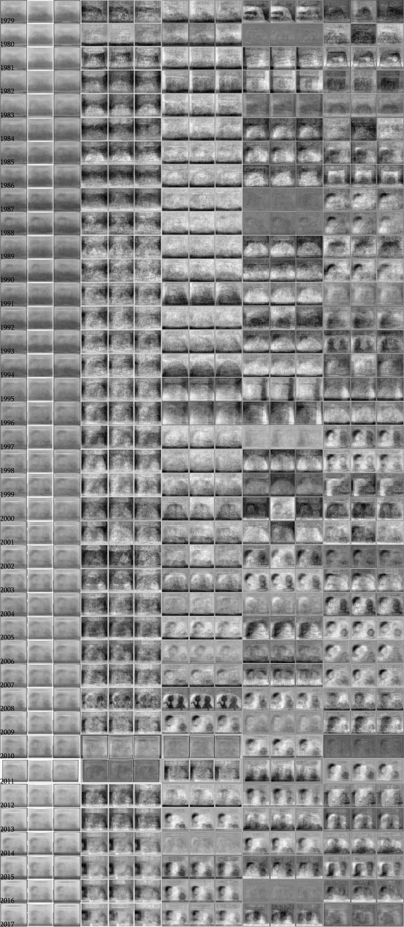
{A 4 by 39 table of monochrome pictures that look vaguely like Garfield strips}
The author writes:
This picture shows the average of all non-Sunday (non-leap day) Garfield strips in monochrome from the years 1979 to 2017, followed by the first four principal components. To explain what that means, I guess it's time for a long scientific annotation. I'll try to do my best to make it easily understandable:
Principal Component Analysis (short PCA) is a mathematical method invented to better analyse multi-dimensional variable distributions. As an example, imagine you were measuring the wing span, beak length and weight of every bird that passed through a forest, from the shortest wren to any of Haast's eagles that might happen to pass by (the moa the merrier). Each data point you'd be writing down would consist of three numbers, the two lengths and the weight, and if you wanted to plot that cloud of data points, your diagram would therefore need three axes.
You can do normal statistical analysis on such multi-dimensional distributions, like calculating the mean, which is just the mean calculated for all three components separately. But when it comes to the deviation from that mean, calculating it for every component separately is not as descriptive as it is for a one-dimensional distribution. To take our bird example, we'll have large deviations for all three of our variables, wing length, beak length and weight. But those three are probably not independent. Even though there can be large beaks and short wings, probably none of the birds in your garden had a metre-long beak, four-centimetre wings, and weighed a pound. Instead, there were small birds, which had small wings, small beaks and weighed little, and large birds, with long beaks, long wings and some weight. The three separate distributions don't paint the full picture.
Thus the need for an algorithm to try and find some independent distributions, whose variances give a better idea about what kind of things flutter through your garden. One such algorithm is the PCA, which mathematically works as follows. If you're not good with or interested in mathematics, just skip two paragraphs.
First, we create a so-called covariance matrix, which is a table for which we can imagine the row and column labels to be the dimensions of our distribution, so for our bird example "wing length", "beak length" and "weight". In each cell the entry is the covariance, which is how much those two measurements vary together. We find that by subtracting the mean value from all our data, and then multiplying the two values we're comparing for each data point, and then finding the mean for that distribution. We also do that for the cells where row and column label are the same - in this case the covariance is just the normal variance of the distribution.
And then we find the eigenvectors of that matrix. This might seem difficult to visualize if one considers eigenvectors on the basis of passing through a function of some kind, because it's difficult to imagine what kind of vector we're giving to that matrix to find a vector of equal direction. But mostly, we do this because of an important property of eigenvectors: they're perpendicular to each other. And what's more, if we turn and flip our coordinate system for our data point so that we're measuring everything as multiples of the eigenvectors, instead of our original set of measurements, then our covariance matrix will have entries of 0 in all cells which aren't on the diagonals, meaning our distributions are independent, which is exactly what we've been looking for. As a bonus, our diagonal entries, which are also the eigenvalues, are the variances of the distribution in the direction of the eigenvector, so we don't even need to recalculate to find those.
There is a neat way to visualize the process if you're not interested in matrix algebra: we take our multi-dimensional cloud of data, and look in which direction it varies the most. This is our first principal component (= first eigenvector), and the one with the greatest variance. We write it down, then squish the cloud flat along that direction, so it now has a dimension less. Then we repeat the process, finding the direction it varies the most in, then squishing it flat, until we have all our data squished into a single point. Then our list of directions are the principal components of our distribution.
If we take useful data, there is a good chance that some of those principal components have some kind of intuitive label, like the example of "size" given above for birds, which would be a vector having positive entries for all three values. In layman's terms, if a bird's size increases, wing span, beak length and weight all increase. Another principal component might be labeled "flight ability": as this component goes up, wing length increases and mass decreases.
And there, we can already see a use emerge for our PCA. By finding these principal components, we have found a compound measurement that can tell us more about the structure of the data than the single measurements, and because we know the variance along each of them, we also know how important they are. If birds vary a lot in size and the other two directions little, then to determine what species a new bird is, it's probably enough to find out its size.
For our three variables, that might not seem useful, but imagine having a hundred variables for each data point. Or 26700. Imagine your data point is actually a picture of a human face, with RGB pixel values given for each pixel. Now, PCA allows us to figure out how faces actually differ from another, in a way that we can teach a computer, by feeding it a large database of faces and making this analysis. Some of those principal values might look to us like they could have labels, like for example "age". If people get wrinkly, those wrinkles appear in about the same spots for every face, and therefore every face gets darker in the same parts with age. Or with a big nose, the shadow of the nose wanders outwards, meaning some pixels at the outside edge of the nose get darker, and those on the inside brighter.
There will be hundreds of principal components from our program (due to a fun mathematical property of the PCA, there can be at most as many principal components as the minimum of dimensions and data points. If we feed it less faces than each face has pixels, that will limit the number of components, not our resolution), but some will have really low variances. In fact, from a database of 500 faces, only 40 principal components might be needed to reconstruct any face with reasonable accuracy. And that's good if we want to use that for face recognition, by passing an unknown picture into the database. Instead of having to compare it pixel by pixel with each face in our library, we measure it along our 40 or so principal components and only have to compare those values. We go from comparing tens of thousands of bytes to comparing about a hundred, a huge leap in efficiency. Also, we can use the PCA, together with human brains, to filter out what's actually important about a face. Imagine a face being lit from the right or the left. One half is therefore darker, the other lighter. This will be a very common variance in the faces, and therefore a high-ranked principal component. But of course, it's not a distinctive feature of a person, what direction they're lit from. So we can tell the program to disregard such components and focus only on the relevant details. We don't need to sit down and figure out by ourselves how a picture changes with the lighting, we just have to look at the PCA and tell the program: "Ignore that one". A lot easier. This face recognition algorithm, by the way, has the name "Eigenface", because of the above use of eigenvectors.
Now, what you see above is this PCA algorithm run over a load of pictures - just not faces, but rather Garfield strips. By how the PCA works, we should get pictures out that tell us how Garfield strips differ from the average, better than a by-pixel standard deviation does (you can see one in SRoMG #1429). I calculated them on my home computer, using my own implementation of the algorithm. The pictures are that small and in monochrome because my copy of Maple refused to handle any sets of data much bigger than the 8357100 matrix entries each year consisted of, and double size would be a factor of 4 and colour a factor of 3 to that size. Funnily enough, however, even though this large amount of data was the maximum I could handle, the calculation of the PCA for all pictures of a year was faster than downloading all the pictures of that year.
So now on to interpreting what we see. There's already been lots written about the progression of averages of Garfield that we see in the first column. Each successive column should now tell us about ways to distinguish Garfield comics from that average. However, it has to be noted that principal components, as vectors, have both positive and negative entries, which got squished into the black-white colour scale of a picture here. Note the colour of the gutter around the pictures, which corresponds to the zero for each principal component, since the gutter doesn't change. Parts that are lighter than that gutter will make the average lighter when added, parts darker will make it darker. We can also subtract that same component, for the opposite effect.
A practical example: look at the second PC column of the year 2016. It shows to the left and right a dark John and Garfield, talking over the Ledge. In between them, if you look closely, you can see a white, ghostly Garfield standing on the same ledge. Now look at the average. If we add that component to the average, we make the John and Garfield blobs on each side of the picture sharper, while we lighten the area in between, making it blend with the (on average brighter) background - we get closer to a "Talking Heads" strip! If we instead subtract the component, we remove the two talking heads and instead add a Garfield in the middle - we get a "Garfield tells us something" strip. Neat!
Now, let us see if we can see other neat things. Take a look at the second column, from 1979 all the way to 2007. In a few years, the component looks different, although in fact a similar-looking component appears at a lower rank (3rd in '94 and 2006 and 4th in '95 and '96). This component has a dark bar at the bottom. We can call this component "Ledgeness". If it's added, we get that dark rectangle at the bottom of the strip that is the Ledge. If we remove it, we get a strip without. Looking at 1982, we can see that when there was no ledge, then Garfield was hanging off a tree branch, as shown by the ghostly outline above.
It's interesting to note that already a week of similar looking strips can create a very strong impression upon the PCA. In 1982, he hung off a tree. In 1979 and 1981, John sat in a car. In 2008, Garfield and Arlene watched the sunset. We also can see that strong statistical outliers have a huge variance and therefore affect the result a lot. The first component of 1979 shows very clearly a silhouette of Garfield in a bright hemisphere. That is from a single strip, 1979-12-14. That strip has two nearly completely black panels in a year with no other night or power outage strips. It's so much of an outlier that it by itself creates the biggest variance and thus gets top spot in the PCA. If we were doing this algorithm with faces, such a result would mean that this is such an atypical picture that it's probably not actually a face.
Now let us look at another component that is easily distinguishable, which I call "Jon's Hair". It first appears in 1987, really blurry and indistinct, and then it's on-and-off until it reappears in 2002 in full force, getting two spots. From then on, it stays around every year, becoming crisper and crisper and rising in the ranking, until it's 2nd place in 2017. Not in every year is it the same axis of "Talking Heads" to "Expiration Dates"; for example in 2006 it's in both signs about Jon and Garfield talking, but in one way Jon is standing upright, and in the other way he's leaning forward.
But look at the principal component that component is losing to in the last four years. It's a picture of Garfield watching TV. That's right. By looking at the first two principal components only, we can tell that most Garfield strips from 2014 to 2017 were of one of three types: Garfield watching TV, Jon on the left talking to Garfield on the right, or Garfield being alone in the middle of the panel. I don't think there can be clearer proof of the declining visual variety of Garfield strips than this. Compare to the '90s, where the first component is so confusing that it's impossible to tell what the strip turns into when you add the component in either direction. Those were, visually at least, the pinnacle years of Garfield.
Onto something different. See the years 2010 and 2011. In those years, the format in which the strips are saved at Garfield's Art Gallery changes, including larger outside gutters. It switches format somewhere in the middle of '10 and switches back early in '11, leaving a clear scar on the 2010 average. But an even clearer one on the principal components. The first component of 2011 and the first two components of 2010 are just about which format the strip is saved in, not telling us anything about what's actually shown there. This shows a disadvantage of the Eigenface algorithm, one that also hobbles its use for face recognition. The PCA only gets pixel values. It can only measure if these pixels get darker or brighter. It can't determine that maybe the best explanation for what changes is that the pixel got moved from a neighbouring position, because that is not a valid operation within the theory. If you turn your head, some pixels move sideways. But looking at it from what pixels get darker or brighter, you'll realize that which of those do depends so much on the face structure that there won't be a clear "Head turned left" principal component.
The solution, as to any "garbage in, garbage out" problem, is to be smarter about what data you pass in. We nowadays have algorithms that can find the important facial features in a picture (eyes, nose, ears, mouth) and find out which coordinates those parts have. We can then place a network of triangles over the face that give us more-or-less its shape in space. And then we can first throw out all pixels not covered by those triangles because they're background and hair and not important for faces, and then - instead of just passing on the picture like this to the PCA - give every pixel a position relative to the triangles, and use those. The effect is that we compare pixels relative to their position to different features. To get back to the example of wrinkles: take crow's feet. They darken the picture at the outer corner of the eyes. Which actual pixels those are depends on where the eyes are, but if we distort the picture first so the eyes are always in the same position, then the crows's feet will be, too.
We are, in effect, splitting the face into its three-dimensional shape, and its texture, and then running the PCA for those, separately or simultaneously however we like (it's unlikely that a pixel value will strongly correlate to a shape). In the space of coordinates, "turn left" is indeed a valid, linear principal component: all points wander left, the nose more, the points on the left side less. This way, we can get a better database of facial components, one that is also easier to read for a human and where we can more easily select what is actually important.
And now you know how Garfield getting boring can teach you about computer face recognition.
[[Original strips: All of them. Well, all non-Sunday, non-leap day strips from 1979 to 2017. I have a lot of pictures on my hard drive now.]]
Original strip: 1979-12-14.
Irregular Webcomic! | Darths & Droids | Eavesdropper | Planet of Hats | The Prisoner of Monty Hall
mezzacotta | Lightning Made of Owls | Square Root of Minus Garfield | The Dinosaur Whiteboard | iToons | Comments on a Postcard | Awkward Fumbles
Garfield and associated character names and likenesses are registered trademarks of Paws, Inc., which does not sponsor, authorise, or endorse this site.
This is a fan-produced parody site. Original comic strips are copyright Paws, Inc. and are used here only as a vehicle for parody.
Original aspects of this work are licensed under a Creative Commons Attribution-Noncommercial-Share Alike 3.0 Unported Licence by The Comic Irregulars. sromgsubmissions@gmail.com