atmospheric physics – 100 Proofs that the Earth is a Globe

46. The Hunga Tonga eruption

There is a fairly straightforward experiment that we could do to establish that the Earth is a globe: Set off an enormous bomb.

Something of explosive power equivalent to 5-10 megatons of TNT. This is around 500 times as powerful as the Hiroshima atomic bomb. Ivy Mike, the first first full-scale thermonuclear hydrogen bomb detonation by the United States would serve nicely, with its yield of just over 10 megatons. The explosion of such a bomb would create a huge shockwave in the atmosphere, which would propagate outwards at the speed of sound in all directions.

This explosive shockwave would create a momentary barometric pressure spike as it passed by weather stations. Nearby stations would see a large pressure spike, while stations thousands of kilometres away would see a spike of the order of a millibar or two. This is strong enough that barometers all over the world should be able to detect the pressure wave passing through the atmosphere. You could then map the arrival time of the pressure wave, emanating in concentric circles from the bomb’s detonation point.

At the point on the Earth antipodal to where the bomb detonated, exactly on the opposite side of the globe, the pressure wave would converge from all directions approximately 16 hours later. This would demonstrate that there is an antipodes, a point on the opposite side of the spherical Earth. This phenomenon of the converging shockwave would not be observed on a flat Earth.

Unfortunately, this experiment is ethically dubious at best.

On 14 January, 2022, the volcano Hunga Tonga erupted explosively, approximately 65 km north of Tonga’s main island of Tongatapu. As I write this a week later, the scale of the destruction and damage to Tonga is still being assessed. According to various estimates, the explosion released somewhere in the range of 5-10 megatons of energy, making it the largest volcanic explosion of the 21st century to date. The eruption and the resulting tsunamis are of course a human tragedy, but they also provide opportunities for knowledge and understanding.

The explosion occurred at 17:15 local time on 14 January (04:15 UTC, 15 January). Soon after, meteorological stations across the world were recording changes in barometric pressure due to the shockwave. The Australian Bureau of Meteorology released this trace of mean sea level pressure changes caused by the eruption.

Barometric pressure traces from six AU stations

Barometric pressure traces from six stations of the Australian Bureau of Meteorology, showing the arrival of the atmospheric pressure wave. (© Bureau of Meteorology, used with permission in accordance with guidelines for the use of Commonwealth intellectual property.)

The figure shows the propagation time delays as the shockwave travels at the speed of sound. Norfolk Island is 1900 km from Tonga and the wave arrived after about 1 hour 50 minutes. This gives the average speed of sound to be around 330 m/s, which is within the expected range. Perth is 6840 km from Tonga and the wave arrived after a little more than 6 hours. This gives the average speed of sound to be around 310 m/s, which is also within the expected variation given pressure and humidity differences.

Australia is relatively close to Tonga, globally speaking. The UK Met Office also released traces of barometric pressure as recorded at a couple of weather stations near Oxford in the UK.

Barometric pressure traces from two stations of the UK Met Office, showing the arrival of the first pressure wave and second pressure wave at Benson and Brize Norton weather stations. (Contains public sector information licensed under the Open Government Licence v3.0)

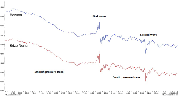
The wave arrived after about 14.5 hours. Given the Tonga-Oxford distance of 16,600 km, this gives a speed of 314 m/s, again well within the expected range. More interesting is the arrival of a second wave a little less than 7 hours later. If we use the same speed of sound, this gives a propagation distance of 24,300 km. This is more than half way around the world. In fact, within the expected range of variation of propagation speed, this is close enough to the distance from Tonga to Oxford, travelling in the opposite direction—the long way around the world.

And this is exactly what we are seeing here. The first recorded wave travelled the shortest path from Tonga to Oxford, while the second wave went in the opposite direction, the long way, and so took 7 hours longer to arrive.

This by itself is strong evidence of the spherical shape of the Earth. But even more dramatic are videos showing propagation of the atmospheric shock wave, as imaged by weather satellites. In the days after the eruption, several meteorologists and atmospheric scientists downloaded publicly available images from geostationary weather satellites. They took infrared images, which show cloud patterns even in night time, and subtracted pairs of images taken at intervals 15 minutes apart, to show the differences between the state of the atmosphere in that time frame.

One resulting video using a satellite over the Pacific Ocean shows the site of the explosion in Tonga and the shockwave rippling outwards in concentric circles on the globe. As the shockwave propagates, you can see it getting weaker.

Video showing Hunga Tonga atmospheric shockwave propagating outwards from Tonga. (Video produced by Dr Mathew Barlow, reproduced with permission.)

A second video uses a satellite over Africa. This shows the shockwave converging on the opposite side of the world. The eruption occurred at latitude 20.550°S, longitude 175.385°W. The antipodal point on the opposite side of the world is thus latitude 20.550°N, longitude 4.615°E, in southern Algeria. And in this video, you can see the shockwave converging on that point in Algeria, and then expanding again, producing the second wave that was later recorded in Oxford. (This video is sped up relative to the first video, to make it easier to see the shockwave propagation, because it is significantly weaker and more difficult to see at the slower speed.)

Video showing Hunga Tonga atmospheric shockwave converging on antipodal point in Algeria then expanding outwards again. (Video produced by Dr Mathew Barlow, reproduced with permission.)

This provides clear visual evidence that the shockwave expands from one point on the Earth’s surface and, after propagating in all directions at approximately the same speed, it converged back to a point on the opposite side of the globe, equidistant from the origin in all directions.

We may not be able to reproduce the experiment with a bomb in good conscience, but nature often provides fascinating ways for us to test our understanding of the world and the universe.

42. Schumann resonances

A waveguide is a structure that restricts the motion of waves, disallowing propagation in certain directions, and thus concentrating the energy of the wave to propagate in specific other directions. An example of a waveguide is an optical fibre, which is basically a long, thin string of flexible glass or transparent polymer. Light entering one end is channelled along the fibre, unable to escape from the sides, and emerges at almost the same brightness from the far end.

Normally light and other electromagnetic waves, as well as other waves such as sound, spread out in three dimensions. As the energy spreads out to cover more space, conservation of energy causes the power to fall off according to the inverse square law: power falls as the reciprocal of the square of the distance from the source.

With a waveguide, propagation of the wave can be restricted to a single dimension so the energy doesn’t spread out, resulting in all of the energy being transmitted to the far end (minus a small fraction that may be absorbed or otherwise lost along the way). Sound waves, for example, can be guided by simple hollow tubes, the sound preferring to propagate along the interior air channel than penetrate the tube walls. This is the principle behind medical stethoscopes and old fashioned speaking tube systems.

Another type of waveguide is a transmission line, which is a pair of electrical cables used to transmit alternating current (AC) electrical power. The cables can simply be parallel wires in close proximity, or a coaxial cable, in which an insulated wire runs down the core of tubular conductor. Domestic AC power has a frequency of 50 to 60 hertz, which is low compared to the kilohertz range of radio frequencies. Transmission lines can carry electromagnetic waves up to frequencies of around 30 kHz. Above this, paired wires start to radiate radio waves, so they become inefficient and a different type of waveguide is used.

Radio waveguides are commonly hollow metal tubes. Radio waves travel along the tube, and the conductive metal prevents the waves from leaking to the outside. Such waveguides are used to transmit radio power in radar systems and microwaves in microwave ovens. Anywhere there is a cavity bounded by regions that waves cannot pass through, a waveguide effect can be generated.

A microwave waveguide, which is essentially a hollow metal tube, but precisely machined to optimal dimensions and with high precision connector joints. (Creative Commons Attribution 2.0 image by Oak Ridge National Laboratory, from Flickr.)

Radio waves travel easily through the Earth’s atmosphere, to and from transmission towers and the various wireless devices we use. However the bulk of the Earth is opaque to radio waves; you generally need a mostly unobstructed line of sight, barring relatively thin obstructions like walls.

But there is another region of the Earth that is opaque to (at least some) radio waves. The ionosphere is the region of the atmosphere in which incoming solar radiation ionises the atmospheric gases (mentioned previously in 31. Earth’s atmosphere). It lies between approximately 60 to 1000 km altitude. Since ionised gas conducts electricity, low frequency radio waves cannot pass through it (higher frequencies oscillate too rapidly for the ionised particles to respond).

Opacity of the Earth’s atmosphere as a function of electromagnetic wavelength. Long wavelength (low frequency) radio waves are blocked by the ionosphere (right). Other parts of the electromagnetic spectrum are blocked by other aspects of the atmosphere. (Modified from a public domain image by NASA, from Wikimedia Commons.)

Radio waves with wavelengths longer than about 30 metres—or frequencies below about 10 MHz—are thus trapped in the atmosphere between the Earth’s surface and the ionosphere. This forms a waveguide which can carry so-called shortwave radio signals around the world, alternately bouncing off the ionosphere and the Earth’s surface.

There are also natural sources of low frequency radio waves. Lightning flashes in storm systems produce huge discharges of electrical energy, and the sudden release of this energy generates radio waves. If you’ve ever listened to a radio during a thunderstorm you’ll be familiar with the bursts of static caused by strokes of lightning. Lightning generates broadband radio emissions, meaning it covers a wide range of radio frequencies, including the very low frequencies that are guided by the ionospheric waveguide.

Atmospheric scientists measure the amount of lightning around the world by monitoring tiny changes in the Earth’s magnetic field, of the order of picoteslas, caused as these radio waves pass by. The sensitive detectors they use can detect lighting strikes anywhere on the planet. There are a few specific radio frequencies at which the lightning strikes turn out to be especially strong. The following plot shows the intensity of magnetic field fluctuations as a function of radio frequency.

Measurements of magnetic field fluctuation amplitude vs radio frequency

Measurements of magnetic field fluctuation amplitude versus radio wave frequency, averaged over a year of observation, at Maitri Research Station, Antarctica. (Figure reproduced from [1].)

The first peak in the observed radio spectrum is at 7.8 Hz, followed by peaks at 14.3 Hz, 20.8 Hz, and roughly every 6.5 Hz thereafter. People familiar with wave theory will recognise from the pattern that these are likely resonance frequencies, with a fundamental mode at 7.8 Hz, followed by overtones. A wave resonance occurs when an exact number of wavelengths fits into a confined cavity. The wave propagates and bounces around and, because of the precise match with the cavity size, reflected waves end up with peaks and troughs in the same physical position, reinforcing one another. So at the specific resonance frequency, the wave builds up in intensity, while at other frequencies the waves self-interfere and rapidly die down. These resonance frequencies, which are measured at many research stations around the world, are known as Schumann resonances.

The Irish physicist George Francis FitzGerald first anticipated the existence of Schumann resonances in 1893, but his work was not widely circulated. Around 1950, the German physicist Winfried Otto Schumann performed the theoretical calculations that predicted the resonances may be observable, and made efforts to observe them. But it was not until 1960 that Balser and Wagner made the first successful observations and measurements of Schumann resonances.[2]

What causes the radio waves produced by lightning flashes to have a resonance at 7.8 Hz? Well, radio waves travel at the speed of light, so let’s divide the speed of light by 7.8 to see what the wavelength is: the answer is 38,460 km. If you’ve been paying attention to many of these articles, you’ll realise that this is very close to the circumference of the Earth.

Radio waves with a frequency of 7.8 Hz are travelling around the world in the waveguide formed by the Earth and the ionosphere, and returning one wavelength later to constructively interfere and reinforce themselves, producing a measurable peak in Earth’s magnetic field fluctuations at 7.8 Hz. The resonance peak is broad and a little different to 7.5 Hz (the speed of light divided by the circumference of the Earth) because the geometry of a spherical cavity is more complicated than a simple circular loop – effectively some propagation paths are shorter because the waves don’t all take a great circle route.

Illustration of Schumann resonances in the Earth’s atmosphere. The ionosphere keeps low frequency radio waves confined to a channel between it and the Earth. Waves propagate around the Earth. At specific frequencies the peaks and troughs line up, producing a resonance that reinforces those frequencies. The blue wave fits six wavelengths around the Earth, the red wave fits three. The fundamental frequency Schuman resonance of 7.8 Hz fits one wave. Not to scale: the ionosphere is much closer to the surface in reality. (Public domain image by NASA/Simoes.)

So Schumann resonances are an observed phenomenon that has a natural explanation – if the Earth is a globe.

If the Earth were flat, then any ionosphere above it would be flat as well, and would still form a waveguide for low frequency radio waves. However it would not be a closed waveguide. Radio waves would propagate out the edges and be lost to space, meaning there would be no observable magnetic field resonances at all. And even if there were an opaque radio wall of some sort at the edge of the flat Earth, the size and geometry of the resulting cavity would be different, resulting in a different set of resonance frequencies, more akin to the frequencies of a vibrating disc, which are not evenly spaced like the observed Schumann resonances.

And so Schumann resonances provide another proof that the Earth is a globe.

References:

[1] Shanmugam, M. “Investigation of Near Earth Space Environment”. Ph.D. Thesis, Manonmaniam Sundaranar University, 2016. https://www.researchgate.net/publication/309209580_Investigation_of_Near_Earth_Space_Environment

[2] Balser, M., Wagner, C. “Observations of Earth–Ionosphere Cavity Resonances”. Nature, 188, p. 638-641, 1960. https://doi.org/10.1038/188638a0

31. Earth’s atmosphere

Earth’s atmosphere is held on by gravity, pulling it towards the centre of the planet. This means the air can move sideways around the planet in a relatively unrestricted manner, creating wind and weather systems, but it has trouble flying upwards into space.

It is possible for a planet’s atmosphere to leak away into space, if the gravity is too weak to hold it. Planets have an escape velocity, which is the speed at which an object fired directly upwards must have in order for it to fly off into space, rather than slow down and fall back down. For Earth, this escape velocity is 11.2 km/s. Almost nothing on Earth goes this fast – but there are some things that do. Gas molecules.

Air is made up of a mixture of molecules of different gases. The majority, around 78%, is nitrogen molecules, made of two atoms of nitrogen bonded together, followed by 21% oxygen molecules, similarly composed of two bonded oxygen atoms. Almost 1% is argon, which is a noble gas, its atoms going around as unbonded singletons. Then there are traces of carbon dioxide, helium, neon, methane, and a few others. On top of these is a variable amount of water vapour, which depending on local weather conditions can range from almost zero to around 3% of the total.

Gas is the state of matter in which the component atoms and molecules are separated and free to move mostly independently of one another, except for when they collide. This contrasts with a solid, in which the atoms are rigidly connected, a liquid, in which the atoms are in close proximity but able to flow and move past one another, and a plasma, in which the atoms are ionised and surrounded by a freely moving electrically charged cloud of electrons. The deciding factors on which state a material exists in are temperature and pressure.

Diagram of gas

Diagram of a gas. The gas particles are free to move anywhere and travel at high speeds.

Temperature is a measurable quantity related to the amount of thermal energy in an object. This is the form of energy which exists in the individual motion of atoms and molecules. In a solid, the atoms are vibrating slightly. As they increase in thermal energy they vibrate faster, until the energy breaks the bonds holding them together, and they form molecules and start to flow, becoming a liquid. As the temperature rises and more thermal energy is added, the molecules begin to fly off the mass of liquid completely, dispersing as a gas. And if more energy is added, it eventually strips the outer electrons off the atoms, ionising the gas into a plasma.

The speed at which molecules move in a gas is determined by the relationship between temperature and the kinetic energy of the molecules. The equipartition theorem of thermodynamics says that the average kinetic energy of molecules in a gas is equal to (3/2)kT, where T is the temperature and k is the Boltzmann constant. If T is measured in kelvins, the Boltzmann constant is about 1.38×10^-23 joules per kelvin. So the kinetic energy of the molecules depends linearly on the temperature, but kinetic energy equals (1/2)mv², where m is the mass of a molecule and v is the velocity. So the average speed of a gas molecule is then √(3kT/m). This means that more massive molecules move more slowly.

For example, here are the molecular masses of some gases and the average speed of the molecules at room temperature:

Gas	Molecular mass (g/mol)	Average speed (m/s)
Hydrogen (H₂)	2.016	1920
Helium	4.003	1362
Water vapour (H₂O)	18.015	642
Neon	20.180	607
Nitrogen (N₂)	28.014	515
Oxygen (O₂)	32.000	482
Argon	39.948	431
Carbon dioxide (CO₂)	44.010	411

Remember that these are the average speeds of the gas molecules. The speeds actually vary according to a statistical distribution known as the Maxwell-Boltzmann distribution. Most molecules have speeds around the average, but there are some with lower speeds all the way down to zero, and some with higher speeds. At the upper end, the speed distribution is not limited (except by the speed of light), although very few molecules have speeds more than 2 or 3 times the average.

Maxwell-Boltzmann distribution for helium, neon, argon, and xenon at room temperature. Although the average speed for helium atoms is 1362 m/s, a significant number of atoms have speeds well above 2500 m/s. For the heavier gases, the number of atoms moving this fast is extremely close to zero. (Public domain image from Wikimedia Commons.)

These speeds are low enough that essentially all the gas molecules are gravitationally bound to Earth. At least in the lower atmosphere. As you go higher the air rapidly gets thinner—because gravity is pulling it down to the surface—but the pressure means it can’t all just pile up on the surface, so it spreads ever thinly upwards. The pressure drops exponentially with altitude: at 5 km the pressure is half what it is at sea level, at 10 km it’s one quarter, at 15 km one eighth, and so on.

The physics of the atmosphere changes as it moves to higher altitudes and lower pressures. Some 99.998% of the atmosphere by mass is below 85 km altitude. The gas above this altitude, in the thermosphere and exosphere, is so rarefied that it is virtually outer space. Incoming solar radiation heats the gas and it is so thin that heat transport to lower layers is inefficient and slow. Above about 200 km the gas temperature is over 1000 K, although the gas is so thin that virtually no thermal energy is transferred to orbiting objects. At this temperature, molecules of hydrogen have an average speed of 3516 m/s, and helium 2496 m/s, while nitrogen is 943 m/s.

Diagram of the layers of Earth’s atmosphere, with altitude plotted vertically, and temperature horizontally. The dashed line plots the electron density of the ionosphere, the regions of the atmosphere that are partly ionised by incident solar and cosmic radiation. (Public domain image from Wikimedia Commons.)

While these average speeds are still well below the escape velocity, a small fraction of molecules at the high end of the Maxwell-Boltzmann distribution do have speeds above escape velocity, and if moving in the right direction they fly off into space, never to return to Earth. Our atmosphere leaks hydrogen at a rate of about 3 kg/s, and helium at 50 g/s. The result of this is that any molecular hydrogen in Earth’s atmosphere leaks away rapidly, as does helium.

There is virtually no molecular hydrogen in Earth’s atmosphere. Helium exists at an equilibrium concentration of about 0.0005%, at which the leakage rate is matched by the replacement of helium in the atmosphere produced by alpha decay of radioactive elements. Recall that in alpha decay, an unstable isotope emits an alpha particle, which is the nucleus of a helium atom. Radioactive decay is the only source of helium we have. Decaying isotopes underground can have their alpha particles trapped in petroleum and natural gas traps underground, creating gas reservoirs with up to a few percent helium; this is the source of all helium used by industry. Over the billions of years of Earth’s geological history, it has only built up enough helium to last our civilisation for another decade or two. Any helium that we use and is released to the atmosphere will eventually be lost to space. It will become increasingly important to capture and recycle helium, lest we run out.

Because of the rapid reduction in probabilities for high speeds of the Maxwell-Boltzmann distribution, the leakage rate for nitrogen, oxygen, and heavier gases is much slower. Fortunately for us, these gases leak so slowly from our atmosphere that they take billions of years for any appreciable loss to occur.

This is the case for a spherical Earth. What if the Earth were flat? Well, the atmosphere would spill over the sides and be lost in very quick time. But wait, a common feature of flat Earth models is impassable walls of ice near the Antarctic rim to keep adventurous explorers (and presumably animals) from falling off the edge. Is it possible that such walls could hold the atmosphere in?

If they’re high enough, sure! Near the boundary between the thermosphere and the exosphere, the gas density is extremely low, and most (but not all) of the molecules that make it this high are hydrogen and helium. If the walls were this high, it would stop virtually all of the nitrogen and oxygen from escaping. However, if the walls were much lower, nitrogen and oxygen would start leaking at faster and faster rates. So how high do the walls need to be? Roughly 500-600 kilometres.

That’s well and truly impassable to any explorer using anything less than a spacecraft, so that’s good. But walls of ice 500 km high? We saw when discussing hydrostatic equilibrium that rock has the structural strength to be piled up only around 10 km high before it collapses under its own gravity. The compressive strength of ice, however, is of the order 5-25 megapascals[1][2], about a tenth that of granite.

Compressive strength of ice

Compressive yield (i.e. failure) strength of ice versus confining (applied) pressure, for varying rates of applied strain. The maximum yield strength ranges from around 3 MPa to 25 MPa. (Figure reproduced from [1].)

Ice is also less dense than rock, so a mountain of ice has a lot less mass than a mountain of granite. However, doing the sums shows that an Everest-sized pile of ice would produce a pressure of 30 MPa at its base, meaning it would collapse under its own weight. And that’s more than 50 times shorter than the walls we need to keep the atmosphere in.

So the fact that we can breathe is a consequence of our Earth being spherical. If it were flat, there would be no physically plausible way to keep the atmosphere in. (There are other models, such as the Earth being covered by a fixed firmament, like a roof, to which the stars are affixed, but these have even more physical problems – which will be discussed another day.)

References:

[1] Jones, S. J. “The confined compressive strength of polycrystalline ice”. Journal of Glaciology, 28 (98), p. 171-177, 1982. https://doi.org/10.1017/S0022143000011874

[2] Petrovic, J. J. “Review: Mechanical properties of ice and snow”. Journal of Materials Science, 38, p. 1-6, 2003. https://doi.org/10.1023/A:1021134128038

Share this:

Share this:

Share this: